1. 前言
对于crypto和经济学,笔者确实不是专业的,只能站在业余的角度阅读一下这篇论文,因此只能命名文章标题为“阅读”而非“解读”。
对于这篇论文的两位作者,其实很有意思,想先放在前面做一个介绍。
- Dr. Murray A. Rudd: Satoshi Action Education科学顾问。其学术身份是环境与资源经济学、科学政策研究者。
- Dennis Porter: Satoshi Action Fund 联合创始人&首席执行官,Satoshi Action Education 创始人/负责人之一;长期从事比特币公共政策倡导,频繁在州议会作证。
据悉,二位曾与白宫有联系,坊间流传二人是特朗普智囊团中加密货币的顾问(该说法本人持有疑虑,因为没有什么公开的蛛丝马迹有显露这一点)
文章概括
这篇论文构建了一个自下而上的“数量清算”比特币定价框架——以Epstein–Zin递归1效用刻画跨期偏好,引入随价上升而“节流”的提款函数与采用曲线,并用蒙特卡洛在关键不确定参数上采样来生成至2036年的价格/市值区间,进而指出仅当流动供给跌破约200万枚且执行纪律 α 偏弱时才会集中出现右尾的“超指数/双曲线”上行,并据此给出“到阈值时间”、α估计与抵押占用映射等可观测、政策中性的调节杠杆,以引导“陡峭但有界”的升势。
根据文中的simulation推测,五个关键性指标/变量标明了在2036年四月前后比特币的价格会来到481万2美元关卡。
Introduction
由于比特币(下称BTC)的总量是有限的(在铸币时就固定了数额,不可再生、不可再铸),该资产已经确立了绝对稀缺的特性,近期Doge和XRP的ETF没有获批,而BTC和ETH的ETF早就获批无疑也给所有人一个信号:BTC和ETH两种资产已经经历市场检验,具有稳定性,现在已经被机构与主权资金逐步纳入资产配置,并在基础设施与 L2 推进下,除储值外的支付/跨境等用途也在增强。
之前的文章很多都是研究比特币的价格走势,往往是直接从金融角度来切入,很少有从“供需关系”角度来切入分析的,这篇文章就要从这个角度来分析比特币的未来走势。作者前作发现当流动供给跌破约 200 万枚时,机构的温和净买入即可触发极陡峭上涨,但受三类不确定性限制:
- 真实的长期锁定/丢失量
- 若干关键参数的函数形式与分布
- 以及缺少“价格越高越难执行”的行为刹车。
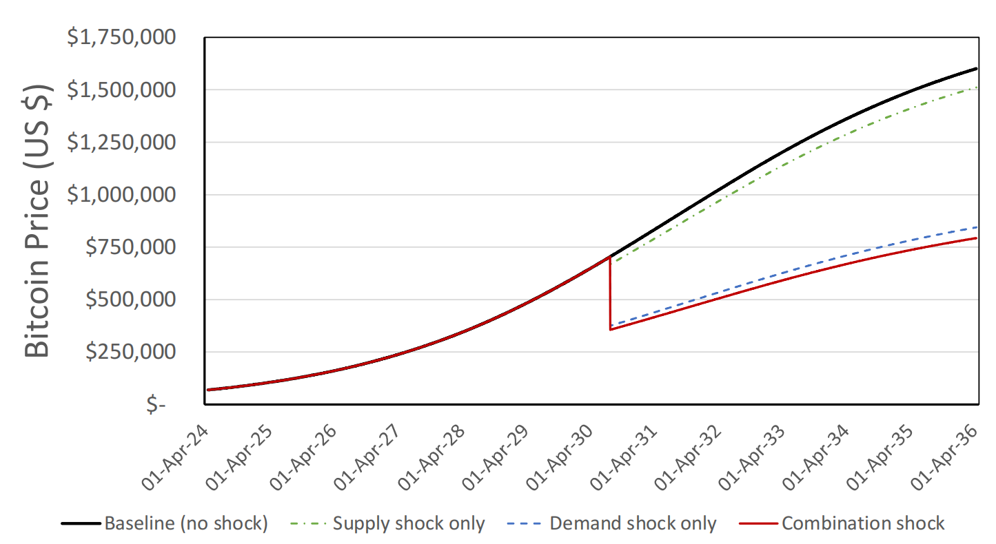
因此,作者据此改进:用Epstein–Zin递归效用替换CES3,把“跨期替代 ρ ”与“风险厌恶”解耦;加入随价格上升而自动“节流”的物流式提款函数;并用蒙特卡洛在宽范围抽样,还示范了对日期型冲击(如 2030 年中“量子攻击 Satoshi 钱包”的假设)的反应;总体贡献是一个可随数据滚动再校准、可嵌入外生驱动的第一性原理定价框架。
2. BTC的供需关系分析
这一块主要分析BTC作为商品属性的基本性质,比特币与其他传统的大宗商品存在巨大差异。一方面BTC总共2100万枚,虽然算力确实在上涨,但是这仅仅影响挖矿的难度(这个在PoW4中叫做difficulty),并不能新增供给的总量。另一方面BTC有出块奖励规则:每210000个区块减半一次,现在挖出一个区块是3.125 BTC的奖励(2025)。2024-04-20 第四次减半后日产出约 450 枚,至 2025-07-29 已挖出约 1,990 万枚、剩余约 110 万枚将在未来一个多世纪逐步释放。这一结构意味着“供给近乎完全无弹性”,价格主要由需求侧推动。
在流动性方面,比特币从交易所转出、进入冷钱包,往往意味着长期甚至永久HODL,从而退出“可流通”池。headline 的“已发行总量”会高估真实流动性:例如约 96.8 万枚被认为属于中本聪早期挖矿、从未移动;丢失币估算在 157 万至 370 万之间,因此,可用于交易的有效存量实际上远低于 1,990 万。同时,链上行为数据显示“存放超过 155 天”的币再度回流市场的概率很低,2025年中估算的“非流动”存量已达约1440 万,对应可流通约300万。
市场需求方面,美国现货比特币 ETF 合计托管约 125 万枚,约占总量 5.9%,其中黑石产品单独就持有 73 万枚以上;在一百多家上市公司中,持有合计超 92.3 万枚,仅微策略(MicroStrategy)一家公司就持有 60.7 万枚;部分矿企选择“囤币不卖”;主权与主权基金也开始配置或讨论战略储备。这些主体的持续买入对可流通供给形成稳定“下水道”。
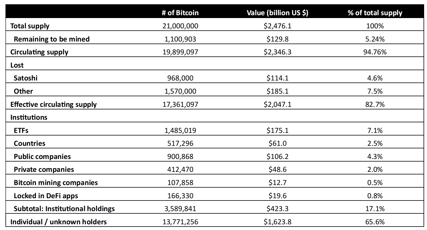
Figure 1. 市场需求分析与比特币Distribution
市场净流出方面,作者汇总了 2025 年上半年的链上与资金流:交易所 30 日均净流出约 2,000 枚/日,单日峰值曾超过 29,000 枚;同期长期持有者群体继续扩大,暗示被提走的币大多“长时间不回”。再加上 ETF 日均约 2,900 枚的净申购、企业定投与主权/机构间歇性大额买入,论文认为每日从“可流通池”中抽走 6,000 枚甚至以上“完全可想见”,这也解释了为什么当可流通存量逼近 200 万枚时,价格会出现非线性上行的脆弱性。
3. 建模与实验
第三节建模了一个实验,详细讲述了文章使用的建模方法,包括用的什么数学公式/框架/模型 (some formula …) 这一块暂时不想详细分析,我们直接看结论。
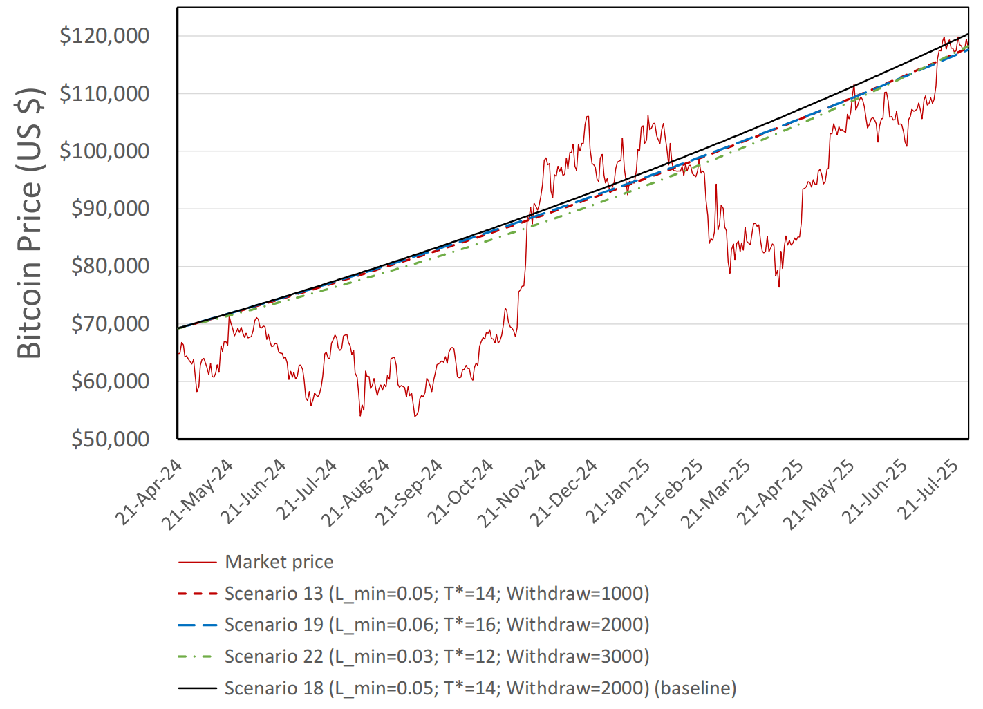
Figure 2. 不同情景实验组拟合BTC价格走势图
对于Scenario 18这一组实验,拟合效果大致是最理想的。以此作为后续灵敏度分析的baseline。当然,一共是有很多种Scenarios的,只不过在这里仅仅展示了其中具有代表性的四组而已。2036-04-16 的市值约29–41万亿美元;年化回报 29–33%。
按照这个模型来预测,“100 万美金/枚”的里程碑节点,大致落在 2030-08 到 2032-02 之间。
ρ在文章中指代“跨期替代”的因子。在ρ=0.5这一组数据中,预测是最早到达100万美元关口的(表格中数据显示在2030年1月27日)最晚的预测是2032年5月19日才会到达。
流动性方面,到 2036 年收官,各曲线仍保留大于7百万枚的流动供给,远高于会触发“失控式上冲”的稀缺阈值。
qbase:日均从流动池抽走,是否影响踩踏阈值?
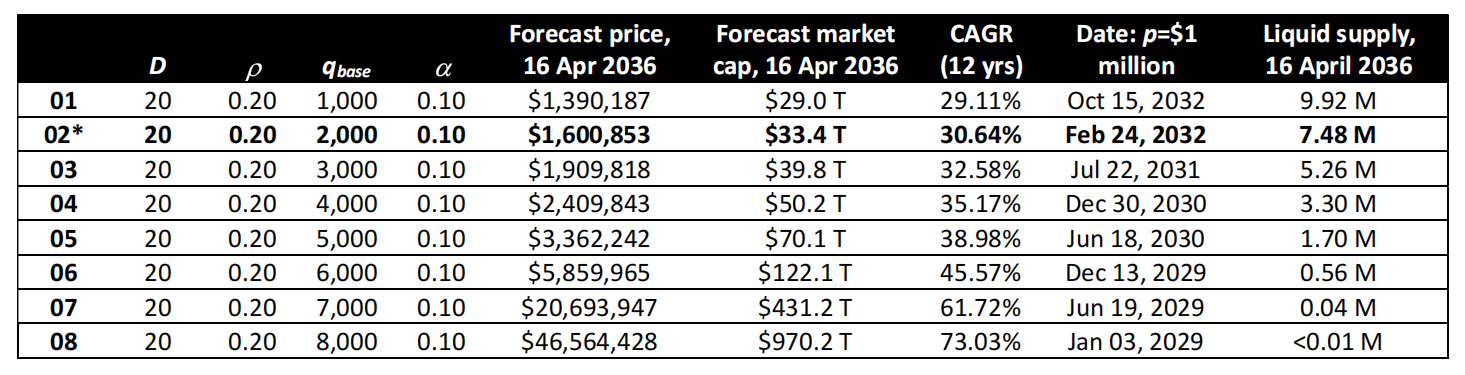
在 D=20,α=0.10 下,qbase从 1,000→5,000:2036-04 价格从 139 万→336 万美元,对应流动供给从 9.9M→1.7M;当 qbase≥6,000 时,2036 年前就会跌破 ~200 万枚“稀缺阈值”,路径开始呈现近失控式上扬:
- 6,000:价格 586 万、流动供给仅 56 万
- 7,000:价格 2,069 万、供给约 4 万
- 8,000:价格 4,656 万、几乎无流动供给
α与qbase的相图边界
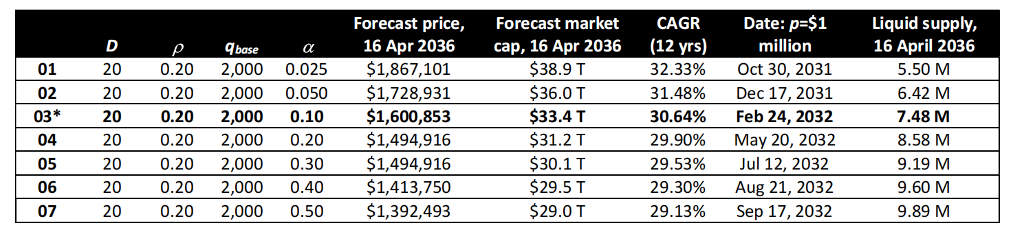
Figure 5. q_base与alpha叠加影响
-
当 qbase=2,000,α 每上调 0.025–0.050,2036年价位大致下降约 14 万美元;α=0.025 时价格约 187 万、流动供给 5.5M;α=0.50 时价格约 139 万、供给 9.89M。
-
若把 qbase翻倍到 4,000 且 α=0.025,会出现流动供给“几乎耗尽”的失控区(100 万美金阈值在 2030-06-20),而把 α 提到 0.05 则能把流动供给抬回 1.55M、但 2036 年价仍高达 352 万。
-
qbase=8,000 时,只要 α<0.10 几乎处处失控;即便 α=0.20,2036 年也给出 517 万/年化 44% 的高位,且仅余 72 万枚流动供给。
总体边界:当每日抽走 ≥4,000 且 α<0.05,或每日 8,000 且 α<0.10,易出现失控;
即使未越界,只要把流动供给压到约 200 万枚以下,价格就会显著加速并更快跨越百万元的台阶。
What about Satoshi Sale?
文章还分析了:假如中本聪钱包突然复活,并且全部抛售了应该怎么办?
在流动性仍“宽松”时(q_base 低),单日-5%~-10% 量级可被市场吸收;
但当日均抽走把流动供给磨到 ≈200 万以下时,同样的 96.8 万枚抛压会引发非线性崩跌(例如 q_base=8,000 条件下一天-38.5%),其危害更取决于当前流动性而非绝对抛售量。
4. Further Discussion
比特币的“路有多陡”,看的是流通盘有多薄、买盘有多“守纪律”、以及外部需求有多猛;一旦可交易的那点“浮动筹码”被抽到差不多两百万枚以下,价格很容易走成非线性的大坡。
文章分析了三个因素:流动供给规模、执行节流α、需求增速D,这三者并列为决定路径的联合风险因子:只要“薄浮动+弱节流”相遇,就容易出现非线性、甚至“近双曲线”的上冲;
反之,价格越涨越会卡住提款(α提高),则多为“陡峭但有界”的上行。
想像市场里有个“水桶”,桶里装的是能在交易所/场内流转的比特币(我叫它“浮动筹码”)。价格涨跌,更多是在比拼这个桶被抽水的速度。如果抽水太快、加水太慢——也就是浮动筹码变“很薄”——哪怕只是普通买单,
也会把价格抬得更快更猛。作者的经验阈值是:当可流通的存量被磨到大约两百万枚以下时,市场进入“容易失控加速”的区间。
决定这件事,有三个关键因素:
- 浮动筹码的厚薄:币在交易所余额越少、长期不动的越多,浮动筹码就越薄。
- 买入“守不守纪律”:“节流” α的概念来描述——越涨越慢买、按预算买而不是按“枚数”买,这就像给大买家装了速度限制器;反过来,如果不节流,价格越涨越想抢,那就更容易把桶抽干。
- 外部需求的猛度:ETF、公司和主权资金的持续买入,会把“愿意持有比特币”的人群基数提高一挡,相当于把整个市场的胃口做大。
一个常见误解被纠正了: 不是“需求越猛越容易失控”。
在需求很猛的世界里,大买家反而更容易切换到“有纪律的买法”,比如按预算/按节奏买,于是能“保住库存”,让上行看起来“陡峭但有界”。真正危险的是需求温和但长期不节流:价格初期涨得不快,大家有更久的时间把币提走、锁仓,长此以往把浮动筹码磨薄,等到某天来一波普通买盘,反而容易引发非线性上冲。
期货、期权、ETF、抵押再质押等,会在一段时间里延缓稀缺(因为很多人拿到了价格敞口,却没动现货)。但在压力时刻(基差挤压、保证金吃紧),这些管道会把库存紧张瞬时传回现货。
作者同样承认了自己建立的模型并不能完全准确的预测,现在测浮动筹码和节流强度都不完美,衍生品与再质押的影响还没完全结构化进模型。
右尾(原文图中可见的那种夸张的加速上涨)是在特定状态下才会出现的条件事件。
Reference
1. Preface
I’m honestly no professional when it comes to crypto or economics, so I can only read this paper from an amateur’s perspective, which is why I’ve titled this post a “reading” rather than an “interpretation.”
The paper’s two authors are actually quite interesting, so I’d like to introduce them up front.
- Dr. Murray A. Rudd: Scientific advisor at Satoshi Action Education. Academically, he is a researcher in environmental and resource economics and in science policy.
- Dennis Porter: Co-founder & CEO of Satoshi Action Fund, and one of the founders/leaders of Satoshi Action Education; he has long been engaged in Bitcoin public-policy advocacy and frequently testifies before state legislatures.
Reportedly, the two have had ties to the White House, and rumor has it that they serve as crypto advisors in Trump’s brain trust (I have my doubts about this claim, since there is no publicly visible trace of evidence pointing to it).
Summary of the Paper
This paper builds a bottom-up “quantity-clearing” Bitcoin pricing framework: it uses Epstein–Zin recursive1 utility to characterize intertemporal preferences, introduces a withdrawal function that “throttles” as prices rise together with an adoption curve, and uses Monte Carlo sampling over the key uncertain parameters to generate price/market-cap ranges through 2036. It then shows that right-tail “super-exponential/hyperbolic” rallies cluster only when the liquid supply falls below roughly 2 million coins and execution discipline α is weak, and on that basis proposes observable, policy-neutral levers, such as “time to threshold,” α estimates, and collateral-encumbrance mapping, to steer the rise toward one that is “steep but bounded.”
Based on the paper’s simulations, five key indicators/variables suggest that Bitcoin’s price will reach the USD 4.81 million2 mark around April 2036.
Introduction
Because the total supply of Bitcoin (hereafter BTC) is finite (the amount was fixed at issuance and can be neither replenished nor re-minted), the asset has established itself as absolutely scarce. The recent failure of the Doge and XRP ETFs to win approval, while the BTC and ETH ETFs were approved long ago, undoubtedly sends everyone a signal: BTC and ETH have been tested by the market and have proven stable. They are now gradually being incorporated into the asset allocations of institutions and sovereign funds, and, driven by advances in infrastructure and L2s, their use cases beyond store of value, such as payments/cross-border transfers, are also growing.
Many earlier studies examined Bitcoin’s price trends, usually approaching them directly from a financial angle; few analyzed them from a “supply and demand” perspective, and this paper sets out to analyze Bitcoin’s future trajectory from exactly that angle. The authors’ previous work found that once the liquid supply falls below about 2 million coins, modest net buying by institutions is enough to trigger an extremely steep rally, but that finding was limited by three kinds of uncertainty:
- The true amount of coins that are locked up long-term or lost
- The functional forms and distributions of several key parameters
- And the lack of a behavioral brake whereby “the higher the price, the harder it is to execute.”
Accordingly, the authors made the following improvements: they replaced CES3 with Epstein–Zin recursive utility, decoupling “intertemporal substitution ρ” from “risk aversion”; added a logistic withdrawal function that automatically “throttles” as prices rise; used Monte Carlo sampling over wide ranges; and also demonstrated the model’s response to date-specific shocks (such as a hypothetical “quantum attack on Satoshi’s wallets” in mid-2030). The overall contribution is a first-principles pricing framework that can be recalibrated on a rolling basis as new data arrive and can incorporate exogenous drivers.
2. Analysis of BTC Supply and Demand
This section mainly analyzes the basic properties of BTC as a commodity, and Bitcoin differs enormously from other traditional commodities. On the one hand, there are only 21 million BTC in total. Although hash power has indeed been rising, this only affects the mining difficulty (known as difficulty in PoW4) and cannot increase the total supply. On the other hand, BTC follows a block reward rule: the reward halves every 210,000 blocks, and mining a block currently earns 3.125 BTC (as of 2025). After the fourth halving on 2024-04-20, daily issuance is about 450 coins; as of 2025-07-29, about 19.9 million coins had been mined, and the remaining roughly 1.1 million will be released gradually over more than the next century. This structure means that “supply is almost perfectly inelastic,” and the price is driven mainly by the demand side.
In terms of liquidity, Bitcoin that moves off exchanges and into cold wallets usually signals long-term or even permanent HODLing, and thus exits the “circulating” pool. The headline “total issued supply” overstates true liquidity: for example, about 968,000 coins are believed to come from Satoshi Nakamoto’s early mining and have never moved, and lost coins are estimated at between 1.57 million and 3.7 million. As a result, the effective stock available for trading is actually far below 19.9 million. Meanwhile, on-chain behavioral data show that coins “held for more than 155 days” have a low probability of flowing back into the market; the “illiquid” stock was estimated at about 14.4 million in mid-2025, corresponding to roughly 3 million liquid coins.
On the demand side, U.S. spot Bitcoin ETFs together hold about 1.25 million coins in custody, roughly 5.9% of the total supply, with BlackRock’s product alone holding more than 730,000; more than a hundred listed companies together hold over 923,000 coins, with MicroStrategy alone holding 607,000; some miners have chosen to “hoard rather than sell”; and sovereigns and sovereign wealth funds have also begun allocating to Bitcoin or discussing strategic reserves. The continuous buying by these entities acts as a steady “drain” on the liquid supply.
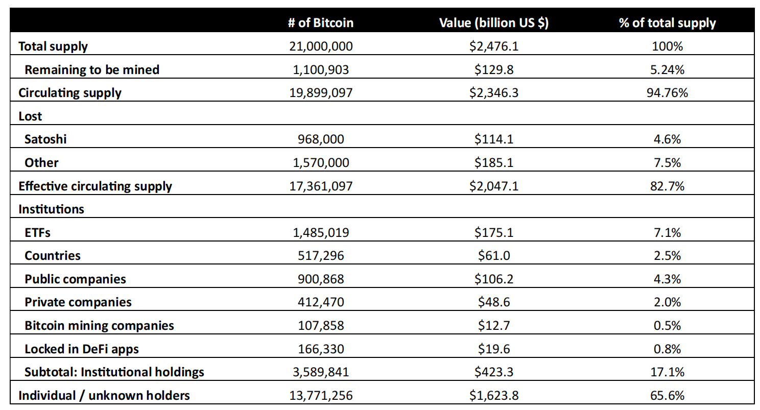
Figure 1. Market demand analysis and Bitcoin distribution
As for net market outflows, the authors compiled on-chain and fund-flow data for the first half of 2025: the 30-day average net outflow from exchanges was about 2,000 coins per day, with single-day peaks that once exceeded 29,000 coins; over the same period, the cohort of long-term holders continued to grow, suggesting that most withdrawn coins “won’t come back for a long time.” Adding in ETF net subscriptions averaging about 2,900 coins per day, corporate dollar-cost averaging, and intermittent large purchases by sovereigns/institutions, the paper considers it “entirely conceivable” that 6,000 or more coins are drained from the “liquid pool” every day. This also explains why, as the liquid stock approaches 2 million coins, the price becomes vulnerable to a nonlinear upswing.
3. Modeling and Experiments
Section 3 builds a model for an experiment and describes the paper’s modeling approach in detail, including which mathematical formulas/frameworks/models it uses (some formula …). I don’t want to analyze this part in detail for now, so let’s go straight to the conclusions.
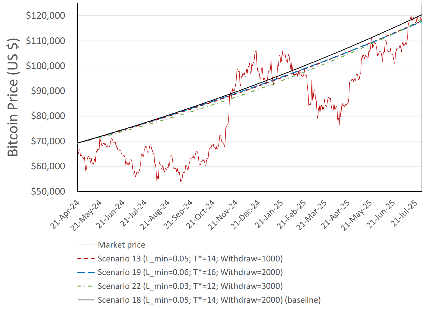
Figure 2. Fitted BTC price trajectories for different experimental scenarios
The Scenario 18 experiment gives roughly the best fit, so it serves as the baseline for the subsequent sensitivity analysis. Of course, there are many Scenarios in total; only four representative ones are shown here. The market cap on 2036-04-16 is about USD 29–41 trillion, with annualized returns of 29–33%.
According to this model’s forecast, the “USD 1 million per coin” milestone falls roughly between 2030-08 and 2032-02.
In the paper, ρ denotes the “intertemporal substitution” factor. The ρ=0.5 case predicts the earliest arrival at the USD 1 million mark (January 27, 2030, according to the table), while the latest prediction has it arriving only on May 19, 2032.
In terms of liquidity, by the end of the horizon in 2036, every curve still retains more than 7 million coins of liquid supply, far above the scarcity threshold that would trigger a “runaway surge.”
qbase: Does the average daily drain from the liquid pool affect the stampede threshold?
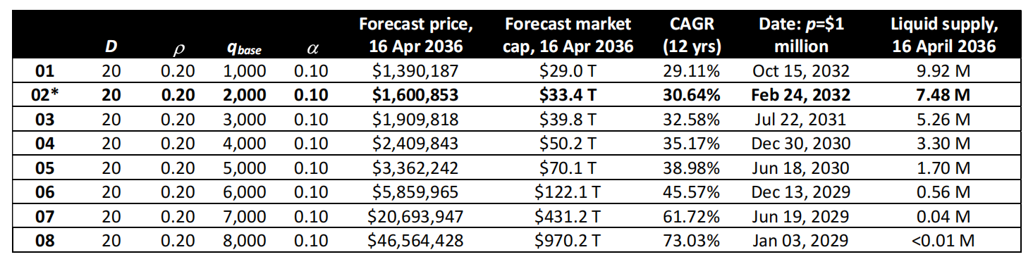
Figure 4. Effect of q_base
With D=20,α=0.10, as qbase goes from 1,000→5,000, the 2036-04 price rises from USD 1.39 million→3.36 million, while the liquid supply correspondingly falls from 9.9M→1.7M; when qbase≥6,000, the liquid supply drops below the ~2 million-coin “scarcity threshold” before 2036, and the path begins to show a near-runaway rise:
- 6,000: price 5.86 million, liquid supply only 560,000
- 7,000: price 20.69 million, supply about 40,000
- 8,000: price 46.56 million, virtually no liquid supply
Phase-diagram boundary between α and qbase
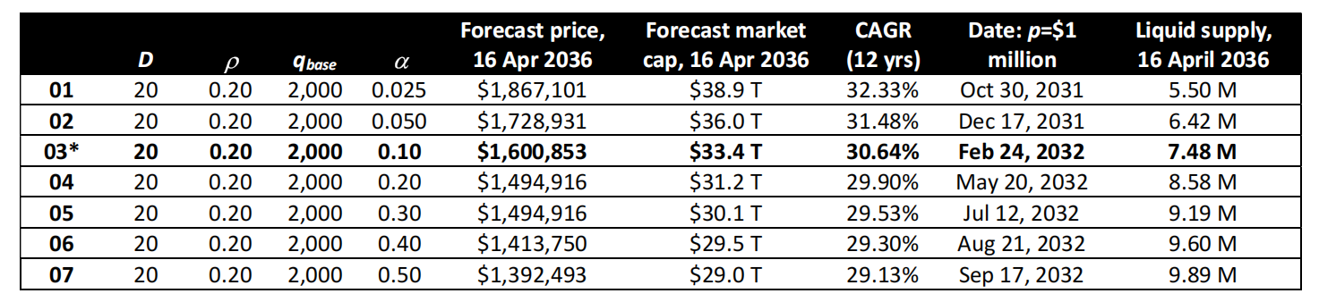
Figure 5. Combined effect of q_base and alpha
-
When qbase=2,000, each 0.025–0.050 increase in α lowers the 2036 price by roughly USD 140,000; at α=0.025 the price is about 1.87 million with 5.5M of liquid supply; at α=0.50 the price is about 1.39 million with 9.89M of supply.
-
If qbase is doubled to 4,000 with α=0.025, the model enters a runaway zone where the liquid supply is “nearly exhausted” (the USD 1 million threshold is reached on 2030-06-20), whereas raising α to 0.05 lifts the liquid supply back to 1.55M, though the 2036 price is still as high as 3.52 million.
-
At qbase=8,000, virtually every run goes out of control as long as α<0.10; even with α=0.20, 2036 still shows a high of 5.17 million / 44% annualized, with only 720,000 coins of liquid supply left.
Overall boundary: runaway behavior is likely when the daily drain is ≥4,000 and α<0.05, or 8,000 per day and α<0.10;
Even without crossing that boundary, as soon as the liquid supply is pushed below about 2 million coins, the price accelerates markedly and crosses the million-dollar mark sooner.
What about Satoshi Sale?
The paper also analyzes this question: what if Satoshi Nakamoto’s wallets suddenly came back to life and sold everything?
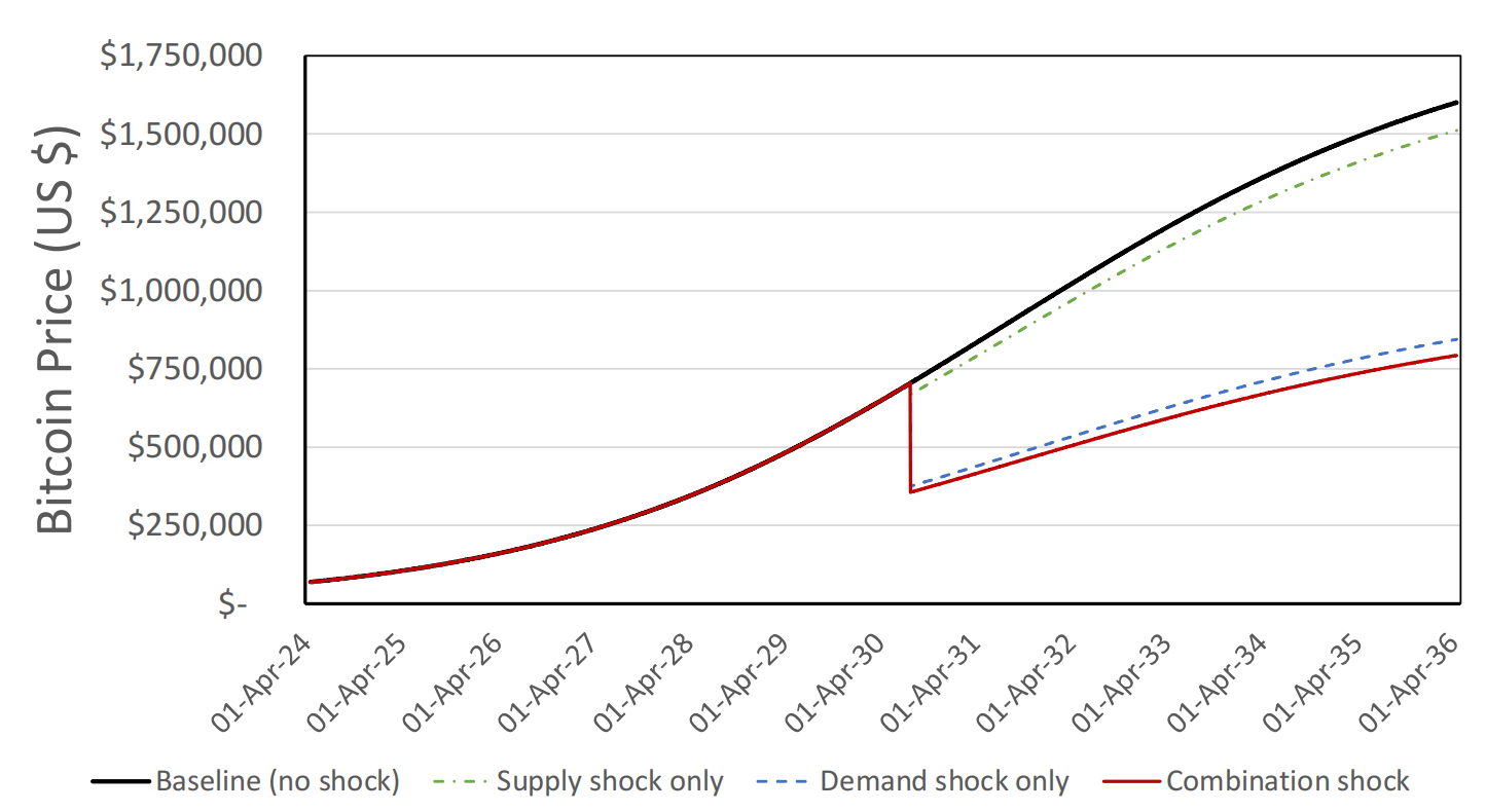
Figure 6. Fitted impact of the sell-off (one of several)
While liquidity is still “loose” (low q_base), a single-day drop on the order of -5% to -10% can be absorbed by the market;
but once the daily drain has ground the liquid supply down below ≈2 million, the same 968,000 coins of selling pressure trigger a nonlinear crash (e.g., -38.5% in a single day under q_base=8,000); the damage depends more on current liquidity than on the absolute size of the sell-off.
4. Further Discussion
How “steep the road” is for Bitcoin depends on how thin the circulating supply is, how “disciplined” the buyers are, and how strong external demand is; once the small pool of tradable “float” is drained to below roughly two million coins, the price can easily turn into a steep nonlinear climb.
The paper analyzes three factors, namely the size of the liquid supply, execution throttling α, and demand growth D, which together act as joint risk factors that determine the path: whenever a “thin float + weak throttling” combination occurs, nonlinear or even “near-hyperbolic” surges readily emerge;
conversely, if rising prices increasingly choke off withdrawals (higher α), the result is mostly a “steep but bounded” climb.
Imagine there’s a “bucket” in the market holding the Bitcoin that can circulate on exchanges and trading venues (I call it the “float”). Price moves are largely a race over how fast this bucket is being drained. If water is pumped out too fast and added too slowly (that is, the float becomes “very thin”), then even ordinary buy orders
will push the price up faster and harder. The authors’ empirical threshold is: once the circulating stock is ground down to below roughly two million coins, the market enters a zone where “runaway acceleration comes easily.”
Three key factors determine this:
- How thick or thin the float is: the smaller the exchange balances and the more coins that sit dormant long-term, the thinner the float.
- Whether buying is “disciplined”: this is described by the concept of “throttling” α. Buying more slowly as the price rises, and buying by budget rather than by “number of coins,” is like fitting large buyers with a speed limiter; conversely, without throttling, the higher the price goes the more eager people are to grab coins, making it much easier to drain the bucket dry.
- The intensity of external demand: sustained buying by ETFs, companies, and sovereign funds raises the base of people “willing to hold Bitcoin” by a notch, effectively enlarging the whole market’s appetite.
A common misconception gets corrected here: it is not the case that “the stronger the demand, the more likely a runaway.”
In a world of very strong demand, large buyers are actually more likely to switch to a “disciplined way of buying,” such as buying by budget or on a set schedule, which lets them “preserve inventory” and makes the ascent look “steep but bounded.” The real danger is moderate demand combined with a persistent lack of throttling: prices rise slowly at first, so everyone has more time to withdraw and lock up their coins; over time this grinds the float thin, until one day an ordinary wave of buying ends up readily triggering a nonlinear surge.
Futures, options, ETFs, collateral rehypothecation, and the like can delay scarcity for a while (because many people gain price exposure without touching spot). But in moments of stress (basis squeezes, tight margins), these channels instantly transmit inventory tightness back to the spot market.
The authors likewise acknowledge that their model cannot make perfectly accurate predictions: current measurements of both the float and throttling intensity are imperfect, and the effects of derivatives and rehypothecation have not yet been fully built into the model’s structure.
The right tail (the kind of dramatic accelerating rally visible in the paper’s figures) is a conditional event that only occurs under specific conditions.
Reference