Our solution is based on the fact that if we for a node in the tree unfold the recursion in the van Emde Boas layout until this node is the root of a bottom tree, then the unfolding will be the same for all nodes of the same depth.
对于一棵高度 H 的大树,作者选择某个节点,顺着 vEB 的规则往下展开递归,直到这个节点本身变成某一层递归调用中的“小树的根”,这就是“unfold until node is root of a bottom tree”。对于树中所有位于相同深度 d 的节点,递归展开到它变成某一层“小树的根”时,展开的形状和布局规则完全一样。
建立搜索表
作者要在隐式的 vEB 布局数组里,给出“当前访问节点在数组中的下标”。为此他们先准备一个按深度预计算的小表:
上一节讲了静态完全二叉树在内存中的四种布局(尤其 vEB 布局)。这一节要把这些静态布局“用在动态树上”:维护一棵动态二叉搜索树,但始终把它嵌入到一棵高度仅为logn+O(1)的静态完全树里,并把静态树按 vEB 布局放进数组。规模翻倍/减半时做一次全局重建。这样既简单(布局基本不变),又能得到和理论最优相匹配的 I/O 复杂度。
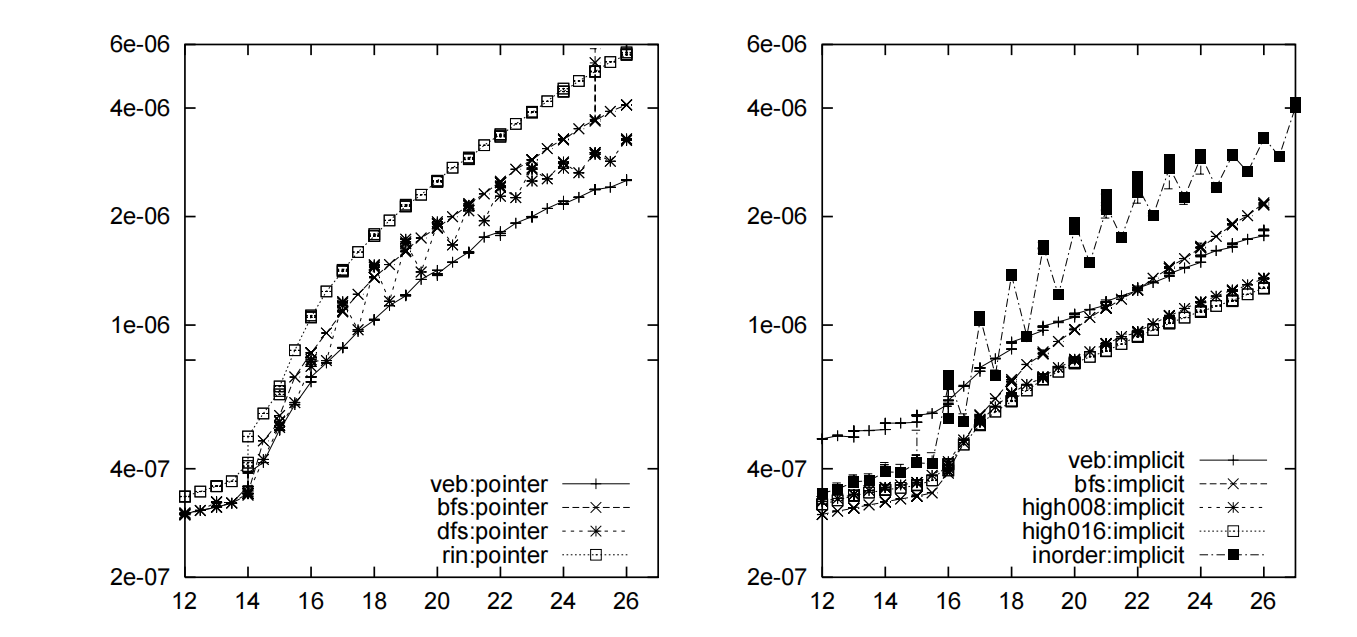
based on pointers的意思是基于指针实现的树。Fig 7中左侧的图就是横向对比集中数据结构基于指针实现的版本。在n比较小的时候,
因为整棵树都在cache里面,所以几种树其实没有太大性能差距(n<14),而在n增大时,BFS每层缺失一次,DFS每两层缺失一次,而vEB每Θ(logBn)层一次,
这根论文中分析的结论几乎一致。
P. van Emde Boas. Preserving order in a forest in less than logarithmic time and linear space. Inf. Process. Lett., 6:80–82, 1977. ↩
H. Prokop. Cache-oblivious algorithms. Master’s thesis, Massachusetts Institute of Technology, June 1999. ↩
S. Chatterjee, V. V. Jain, A. R. Lebeck, S. Mundhra, and M. Thottethodi. Nonlinear array layouts for hierarchical memory systems. In Proceedingsof the 1999 Conference on Supercomputing, ACM SIGARCH, pages 444–453.ACM Press, 1999. ↩
1. Introduction
As chance would have it, while browsing the web today I came across a paper on “cache-oblivious” search trees. What I’ve been learning lately also happens to be connected to cache-oblivious program design, so I decided to take a deep look at this paper.
Aggarwal and Vitter I/O Model
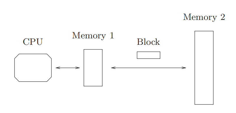
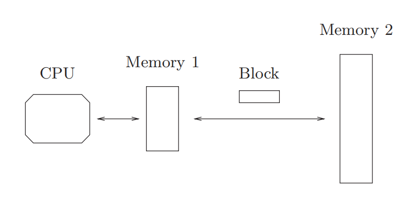
Around 2001, the prevailing I/O model was the Aggarwal and Vitter I/O model. It assumes that memory has two levels, Memory 1 and Memory 2. Memory 2 is regarded as the lower-level memory, with a space whose size can be quantified as M (as shown in Figure 1).
Figure 1. Aggarwal & Vitter I/O Model
The two memories communicate by transferring blocks of B elements. The model’s central point is:
The cost of the computation in the I/O model is the number of blocks transferred
In other words, the model treats the CPU’s accesses to Memory 1 as free, and the total I/O cost equals the number of blocks transferred between the two memory levels. This assumption holds whenever block transfers dominate the running cost.
In fact, from a modern perspective, Memory 2 in this model can simply be viewed as the disk. In other words, when diskdatasize>>memory1size, blocks are frequently swapped in and out of memory1, so disk I/O time far exceeds all other computation time, and the model’s assumption holds.
What is cache-oblivious?
The literal Chinese translation of cache-oblivious reads as “cache-irrelevant”, but no program can run without the cache coming into play, so the right way to understand it here is: cache-oblivious does not mean “unaffected by the cache”, but rather “makes good use of the cache automatically, without needing to know the cache’s parameters”.
A cache-oblivious algorithm/data structure is analyzed in the I/O model (with cost counted as the number of block transfers), but it is designed without knowing the block size B or the available memory M. The analysis holds for any B and M, so it is simultaneously near-optimal at every level of the memory hierarchy; the implementation also doesn’t need to hard-code these hardware parameters, which makes it more portable.
Conversely, a cache-aware algorithm explicitly uses B,M to tune things like a node’s degree and the page size.
Why cache-oblivious?
So why does the notion of cache-oblivious exist at all? With the groundwork above, we can extend the idea like this:
At the Disk-Memory level of the memory hierarchy, if I/O between memory and disk accounts for most of the runtime cost, then our analysis focuses on that stage.
At the Memory-Cache level of the memory hierarchy, if I/O between cache and memory becomes the runtime bottleneck, then our analysis focuses on that stage.
With the cache-oblivious concept, the only things left to consider in our analysis are the size M of the lower level and the size B of the data that can be moved between levels in a single transfer. As a result, we can cover every level of the memory hierarchy: whether it’s Disk-Memory or Memory-Cache, and regardless of the brand or specs of the CPU, memory, or disk, one universal algorithm can fully automatically optimize its detailed strategy.
cache-oblivious makes our algorithms transferable and portable, instead of being custom-tailored to one particular hardware spec and then having to be hand-tuned all over again the next time.
In fact, the overall idea is somewhat similar to the template metaprogramming philosophy of cutlass: auto-tuning. In our later implementation, we will also borrow template metaprogramming to implement cache-oblivious data structures and algorithms.
Some implementations built around cache-oblivious (Before 2001)
The cache-oblivious matrix transpose, FFT, and sorting algorithms proposed by Frigo et al.
The cache-oblivious search tree proposed by Bender et al., whose efficiency is nearly on par with the cache-aware B-Tree.
2. Preliminaries
2.1 Ω,Θ,O
First, let’s go over what these three symbols mean. They appear all over the paper, so we need to sort them out.
In the study of modern data structures and algorithms, the most commonly discussed complexity notation is O, but it represents an upper bound, i.e., the worst case.
There are two other symbols. Let’s first introduce Ω, which represents a lower bound, i.e., the best case:
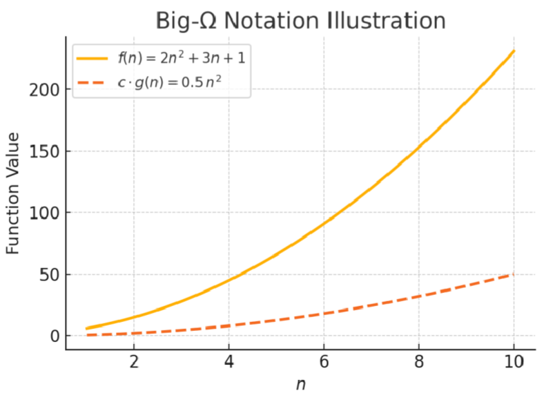
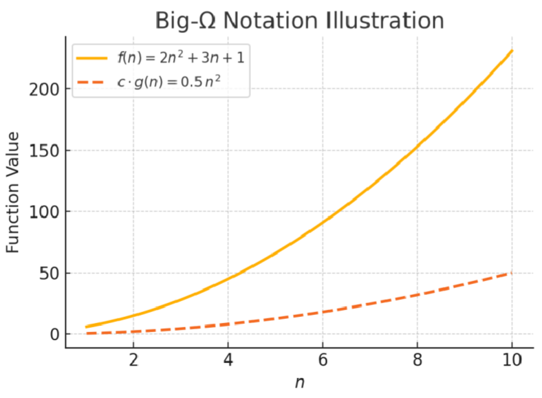
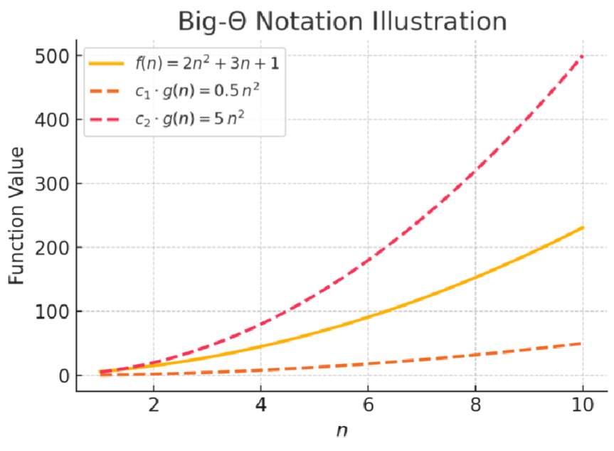
Suppose we have the function f(n)=2n2+3n+1; it is clearly larger than g(n)=0.5n2. Figure 2 shows their graphs:
Figure 2. f(n) vs g(n)
So in this case, we can use Ω to denote its lower bound, which can be written formally as:
f(n)=Ω(n2)
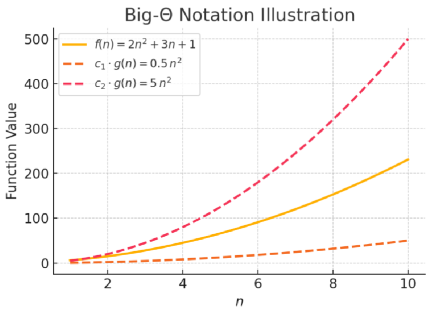
Now, what if a function has both a definite upper bound O and a definite lower bound Ω, as in the situation shown in Figure 3:
Figure 3. The upper and lower bounds of f(n) can be squeezed within the n-squared range
In this case, it can be formalized as: c1g(n)<f(n)<c2g(n). That is, both the upper and lower bounds of f(n) are within n2 complexity. We can then use the Θ notation:
f(n)=Θ(n2)
So whenever you see the Θ symbol later on, you should naturally have this picture in mind: the operation is tightly sandwiched within a certain complexity, with neither the upper nor the lower bound going beyond it.
2.2 van Emde Boas Tree
The data structure proposed by van Emde Boas (hereafter vEB)1 is a dictionary/priority-queue data structure designed specifically for integer keys. Its best-known property is that, with a universe size of U (the key domain is [0,U−1]), it supports all of the following operations in O(loglogU) time:
The design idea of the vEB tree comes from recursively decomposing the universe U:
Split the binary bits of the key into “hi + lo”
Recursively decompose U into U groups, called clusters
Each cluster has size U
There is a summary inside: it records which sub-clusters are non-empty
cluster[0,U−1]: each cluster recursively contains the same vEB structure.
You can look up the complexity analysis of the vEB tree on your own; I won’t go into it here.
2.3 van Emde Boas Layout
The vEB layout2 is a recursive arrangement that “squeezes” a static complete/nearly complete binary tree “into an array”. Its goal is that, without knowing the cache parameters (B,M), root-to-leaf accesses, as well as many local subtree accesses, still automatically enjoy strong locality (which is what makes it cache-oblivious friendly).
Now split it in two, and it turns out that the small trees in the bottom half have the same structure as the tree in the top half:
Top tree 1 Bottom tree 4 2 3 8 9
Then we lay them out recursively. Note that when laying out a bottom tree, if its structure is also complex, we likewise split 2h into 4h+4h and lay it out recursively.
Here, splitting the small tree again gives 4 and 8,9, which can’t be split any further, so we lay them out:
[1,2,3,4,8,9]// Lay them out one after another:[1, 2, 3, 4, 8, 9, 5, 10, 11, 6, 12, 13, 7, 14, 15]
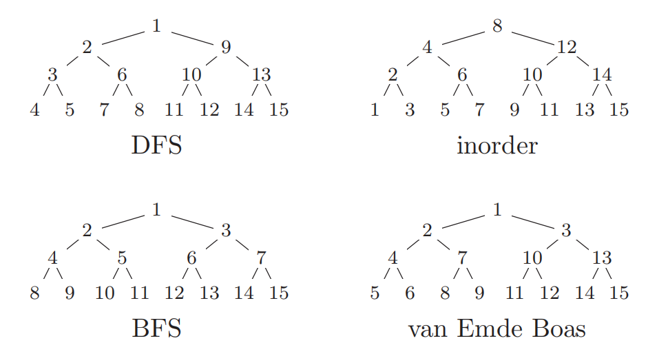
So what would BFS and DFS look like by comparison?
So if we really want to talk about locality, the vEB layout has the best locality and is the most cache-friendly.
The reason we care about layout is that the storage layout significantly affects a program’s performance3.
3. The Paper’s Work
The paper uses the following formal notation to describe the relevant properties:
v: a node
T: Tree, referring to the tree we are currently discussing.
d(v): the depth of a node, i.e., its distance from the root node.
h(T): the height of the tree, generally the distance from the deepest node to the root node.
∣T∣: the number of nodes in the tree, denoted with the absolute-value symbol.
Tv: a subtree rooted at the current node v.
h(v): the height of the subtree Tv.
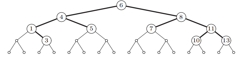
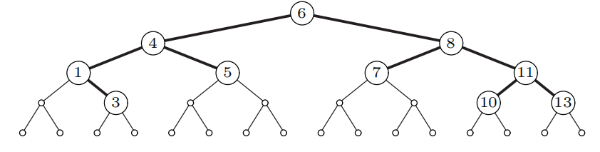
In particular, if a tree T1 can be obtained from T2 by pruning (removing subtrees), we say T1 could be embedded into T2, as shown in Figure 4:
Figure 4. A tree with height=4 and size=10 can be viewed as a pruned version of the complete tree of height=5 obtained by filling it out
3.1 Different Layouts for Serializing a Tree into an Array
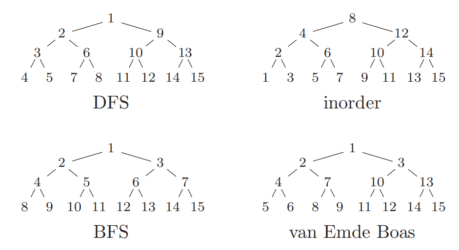
Figure 5. Four different layouts
For the BFS layout, the left and right children are at positions 2i and 2i+1, respectively:
[1, 2, 3, 4, 5]// position 1*2 is 2, position 1*2+1 is 3 these are the left and right children of 1// position 2*2 is 4, position 2*2+1 is 5 these are the left and right children of 2
For the DFS layout, the left and right children are at positions i+1 and i+2h(v)−1, respectively.
[1,2,3,4,5,6,7,8,9,...]// position 1+1 is 2, position 1+2^(4-1) is 9 these are the left and right children of 1: 2 and 9, where 4 is the height of the subtree rooted at the current node: 4// position 2+1 is 3, position 2+2^(3-1) is 6 these are the left and right children of 2: 3 and 6, where 3 is the height of the subtree rooted at the current node: 3
For the in-order layout, the left and right children are at positions i−2h(v)−2 and i+2h(v)−2, respectively. I won’t list an example here, since it isn’t the focus of our discussion.
For the vEB layout, we discussed how it is formed in Section 2.3, and it’s easy to understand here too: it is formed by clustering + recursion.
Our solution is based on the fact that if we for a node in the tree unfold the recursion in the van Emde Boas layout until this node is the root of a bottom tree, then the unfolding will be the same for all nodes of the same depth.
For a large tree of height H, the authors pick a node and unfold the recursion downward following the vEB rules until that node itself becomes the “root of a small tree” at some level of the recursive calls; this is what “unfold until node is root of a bottom tree” means. For all nodes in the tree at the same depth d, when the recursion is unfolded until the node becomes the “root of a small tree” at some level, the shape of the unfolding and the layout rules are exactly the same.
Building the lookup table
The authors want to determine, within the implicit vEB layout array, “the index in the array of the node currently being visited”. To do this, they first prepare a small table precomputed per depth:
For a node at depth d, when the vEB unfolding reaches the round in which this node at depth d has just become the root of a bottom tree:
The size (i.e., number of nodes) of the top tree above it is denoted Top(d),
The size of the small tree below this node is denoted Bottom(d),
D(d) is the depth of the corresponding top tree.
Building such a table only takes O(logn) space, and therefore only O(logn) time.
During a search, we need to maintain two things:
The current position i in BFS numbering (the root is 1, and the left and right children are 2i and 2i+1)
For each depth j along the path, the position Pos[j] in the vEB array of the node already visited at that depth.
Since the binary representation of i, read from the high bits to the low bits, encodes the sequence of “left (0) / right (1)” turns, the low log(T[d]+1) bits of i tell us which bottom tree under the Top Tree of this round of recursion the current node lies in. And since T[d] is exactly of the form 2k−1, “taking the low k bits” is just a bitwise AND (iANDT[d]). The position formula can therefore be written formally as:
Pos[d]=Pos[D[d]]+T[d]+(iANDT[d])×B[d]
Holy shit, I can’t make heads or tails of this; it’s pure gibberish. Let’s work through an example and compute it by hand:
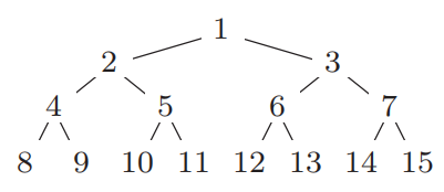
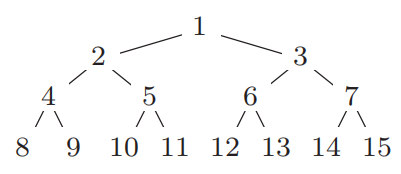
Suppose we have a tree like this.
Figure 6. BFS Layout
The formula for computing Pos is: Pos[d]=Pos[D[d]]+T[d]+(iANDT[d])×B[d]
The per-depth parameter table
d=2: these are nodes 2 and 3. In the second split of the “top half-tree”, they become the roots of bottom trees. In the second round of recursive splitting, the top tree is just {1}, so T[2]=1; each bottom tree contains only the node itself (2 or 3), so B[2]=1; the depth of this top tree (from node 1 to the root, which is also node 1) is D[2]=1
d=3: we’ve reached the third level, i.e., the four nodes {4,5,6,7}. They already became the roots of bottom trees in the first round of splitting. Remember that our splitting rule is: stop once a node becomes the root of a small tree, so the 4 nodes on this level do not take part in the second round of splitting. The top tree is the small tree of height 2 above them, {1,2,3}, so T[3]=3; each bottom tree again has size 3 (4,8,9; 5,10,11; …), so B[3]=3; the depth of the top tree’s root: D[3]=1
d=4: we’ve reached the fourth level, i.e., the 8 nodes {8,9,10,11,...,15}. In the first round of splitting, they end up at the bottom of the small trees; in the second round of splitting, each of them becomes the root of a small tree consisting of just itself, at which point the splitting stops. The top is their parent node (e.g., 4), so T[4]=1, B[4]=1, and the depth of the top root is D[4]=3
Computing the array index in the vEB layout
Node 2: d=2,i=2 (d is the depth, i is the index in the BFS layout)
Pos[2]=Pos[1]+T[2]+(2and1)×B[2]=1+1+0×1=2, so its position in the vEB array is 2
Similarly: 3:Pos[2]=3
Node 4: d=3,i=4 (the depth is 3, and it is at position 4 in the BFS layout)
Pos[3]=Pos[1]+T[3]+(4andT[3])×B[3]=1+3+0×3=4
Similarly: 5:Pos[3]=7
Node 9: d=4,i=9
Pos[4]=Pos[D[4]]+T[4]+(9andT[4])×B[4]=4+1+1=6
Similarly: 8:Pos[4]=5
So in theory, a vEB layout should look like this (in the array):
Following the I/O model described in Section 1, assume that data moves between the two memory levels in blocks. Further assume that in our tree structure, regardless of the layout used, a block can hold at most B nodes.
With the BFS layout, the top log(B+1) levels fit in 2 blocks, but every block read after that contains only one node on the path. The total number of memory transfers is Θ(log(Bn)).
In comparison, the vEB layout needs only O(logBn) memory transfers (note that this O is an upper bound, as analyzed in Section 2.1). Notably, only the vEB layout’s performance can approach that of a B-Tree.
For all four layouts, the number of block transfers for a range query = the number of block transfers for two searches + O(Bk) (k is the number of output elements, and B is the number of nodes a block can hold).
3.3 Search Trees of small height
The previous section covered four in-memory layouts of a static complete binary tree (especially the vEB layout). This section applies these static layouts “to dynamic trees”: maintain a dynamic binary search tree, but always embed it in a static complete tree of height only logn+O(1), and store the static tree in an array using the vEB layout. When the size doubles/halves, do a global rebuild. This is both simple (the layout stays essentially unchanged) and achieves I/O complexity matching the theoretical optimum.
This design has one difficulty: since the tree is embedded in the array of a fixed “static complete tree”, we cannot use rotations, the rebalancing technique that “moves subtrees just by changing pointers”. Instead, the paper controls the height by redistributing/rebuilding subtrees.
3.3.1 Insertion
Notation and invariants:
For the upper bound on the target height, take H≈logn. In the embedded complete tree, a position at depth d(v) has capacity s(v)=2H−d(v)+1−1. The ratio of the actual subtree size ∣Tv∣ to the capacity is defined as:
ρ(v)=s(v)∣Tv∣
We define a sequence of upper density thresholds 0<τ1<τ2<...<τH=1 (note that these τi form an arithmetic progression) and maintain that the root satisfies ρ(root)≤τ1. This design enforces the property H=logn+O(1).
Insertion steps:
First, following the usual Binary Search Tree rules, find the insertion position top-down and create the new node v.
If the depth of v reaches H+1, the prescribed height has been exceeded. We then search bottom-up for the nearest ancestor ω such that ρ(ω)≤τd(w), and do an even rebuild of Tw:
Do an in-order scan to get a sorted array, and place the median at ω;
Recursively fill the left and right halves back into the left and right subtrees (note: this step can be done without an extra array) (first temporarily “push right” the elements, then fill them back in order). This evens out the density of Tw and brings the height back to its previous normal value
The rule for finding ω: if this ancestor’s computed density ρ does not exceed the threshold, start rebuilding from this problem-free ancestor.
Example: rebuilding
Talk alone is still too abstract, so let’s go through an example:
Suppose we have a host complete binary tree with H=3 (at most three levels, with a capacity of 1+2+4=7 nodes).
The capacity at each depth, s(v)=2H−d(v)+1−1:
Depth 1: s=7
Depth 2: s=3
Depth 3: s=1
Then we set the upper thresholds: τ1=0.8,τ2=0.9,τ3=1.
Suppose we now just insert naively (the kind that degenerates into a linked list)
At this point, 40 has gone beyond height 3, making the tree’s height 4.
ρ(d=3)=12=2
ρ(d=2)=33=1, exceeding τ2=0.9
ρ(d=1)=74<0.8, not exceeding τ1
Since the one that doesn’t exceed its threshold is d=1, we rebuild at level d=1:
The in-order sequence at this point is {10,20,30,40}; we choose 20 as the median
Fill the left and right halves back in:
    20
   /  \
 10   30
         \
         40
Example: inserting 50
Now suppose we want to insert 50 as well?
20 / \ 10 30 \ 40 \ 50 ← newly inserted, depth 4
ρ(d=3)=12=2
ρ(d=2)=33=1, exceeding τ2=0.9; there are actually 3 elements, and the capacity it should theoretically hold is s(v)=23−2+1−1=3
ρ(d=1)=75=0.71, not exceeding τ1
At this point, the one without a problem is still the root, d=1, so we rebuild at the root:
[10,20,30,40,50] becomes:
30 / \ 20 40 / \10 50
Example: inserting 60 next
When we then insert 60, even ρ(d=1)≈0.86>0.8; not even the ancestor can satisfy the threshold, so the only option is to rebuild the entire tree and increase its height.
Summary
From the examples above, we can observe that:
Our tree doesn’t have to be completely full to trigger a global rebuild; it may need to be rebuilt even before it is full.
The tree’s capacity, and whether a rebuild is needed, are determined by the parameters τi that we set in advance; in practice, these parameters need to be defined carefully.
Why does this stay stable in the long run?
After a redistribution at v, the actual size of any descendant ω falls within some interval, which is determined by the density and the constants τi. That is, “size = capacity x density”, up to a constant-factor error, which keeps every level from becoming either too crowded or too sparse.
Amortized complexity analysis of insertion
Amortization means spreading the cost evenly across every operation. Some operations trigger a rebuild and some don’t, but for a rebuild we can’t simply count the complexity of the rebuild itself; its cost should be amortized back onto the earlier operations that didn’t trigger a rebuild. Only that is fair.
Time: O(ΔH)=O((1−τ1)log2n)
Block transfers: O(logBn)+O(B(1−τ1)log2n)
3.3.2 Deletion
The Delete operation supports deletion using “density thresholds + local rebuilding” without disturbing the static vEB layout, while still guaranteeing the I/O upper bounds for range queries and searches.
If we simply mark nodes as “deleted” and wait until half of them have been deleted before doing a global rebuild, some regions become very sparse, and range queries can no longer be given a worst-case upper bound on block transfers (i.e., sometimes you have to cross many blocks just to scan a small range). So after a deletion we must rebalance promptly, rather than leaving deletion marks around indefinitely.
Similar to the sequence of upper thresholds we set earlier, the paper here proposes a series of lower thresholds 0<γH<γ2<gamma1<τ1. Note that the bound at the far end is the smallest of the upper thresholds, τ1.
Deletion steps:
First do a standard BST deletion: find, top-down, the node v that holds the element to delete. If v is not a leaf and has a right subtree, find its “successor” and swap with it, repeating until reaching a leaf, then delete that leaf; if there is no right subtree, symmetrically use the “predecessor”.
Rebalance: looking upward from the deleted leaf, find the lowest ancestor ω whose density is back within the valid range γd(ω)<ρ(ω)<τd(ω), then do an even rebuild of the entire subtree Tw. The concrete steps are almost the same as above.
Going further, if we keep deleting, a global height reduction will be triggered.
Amortized cost analysis
Amortized time: O(αlog2n), where α∈min{γ1−γH,1−τ1}
I/O block transfers: searches are still logBn, and updates are amortized O(logBn+Bαlog2n)
3.3.3 Improve Densities
Recap: above, we went through the three techniques the paper proposes: embedding in a static complete tree, the vEB layout, and the density-threshold-based rebuilding scheme.
The next question is: how do we compress the worst-case space from 2n down to
the near-optimal (1+ε)n, without making the I/O upper bounds for searches and range queries any worse?
How do we compress space without knowing B,M?
The paper sets a space usage N and chooses a root density threshold γ1≤Nn≤τ1; once this is violated, it switches to a newN and does a global rebuild. This way, the overall space
is kept strictly on the order of (1+ε)n.
There are then two cases for the value of N:
If N=2k−1, directly use the earlier single “host complete tree” scheme.
Otherwise, write N as a sum of powers of two: N=∑bi2bi=2b1+2b2+2b3+...+2bn
For each bi, build a tree Fi that has just a root ri with no left child, and a complete right subtree Ci of size 2bi−1 attached on the right
Split all the elements into contiguous segments and distribute them onto these Fi.
In memory, arrange them in the order r1,r2,...,rk,C1,C2,...,Ck, with each Ci using the vEB layout.
When searching, first compare against r1,...,rk in order to find which segment Ti the key falls into, then search top-down within Ti. The I/O cost of this is O(Bi+logB(2ib−1))=O(logBN)
Given how often N is changed, the amortized time of global rebuilds is O(ε1), and the I/O cost is O(εB1)
4. Experiments
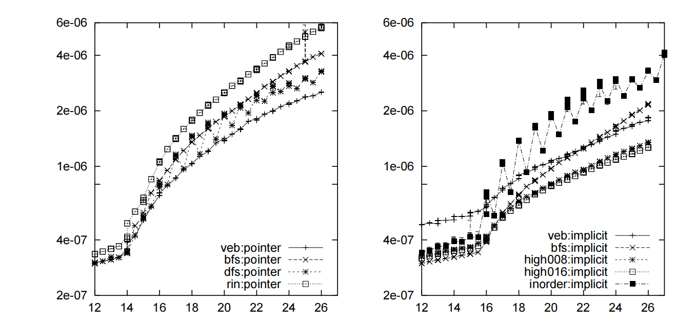
Figure 7. Left: performance of the four layouts with pointer-based implementations; right: performance of the four layouts with array-based implementations
based on pointers means trees implemented with pointers. The left plot in Fig 7 compares the pointer-based versions of several data structures side by side. When n is small,
the whole tree fits in the cache, so there isn’t much performance difference among the trees (n<14). As n grows, BFS incurs a miss at every level, DFS a miss every two levels, and vEB one every Θ(logBn) levels,
which is almost exactly what the paper’s analysis concludes.
The right plot is the experimental analysis of the implicit versions, i.e., the versions with no pointers that rely purely on arrays. Within the cache, address-computation overhead dominates: BFS is the fastest and vEB the slowest (vEB has the most complex addressing).
Once the data exceeds the cache, memory accesses (I/O operations) become the bottleneck, and the high-degree (d=8,16) cache-aware versions are the fastest, since they better match the cache line size. vEB gradually catches up with BFS and eventually overtakes it (at around
n=21∼22). In the end it is only about 50% slower than the high-degree schemes.
The curve for the inorder group fluctuates, especially when n is a power of 2, presumably because limited associativity maps the top nodes to the same cache set.
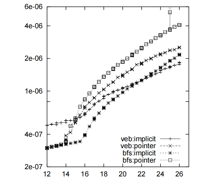
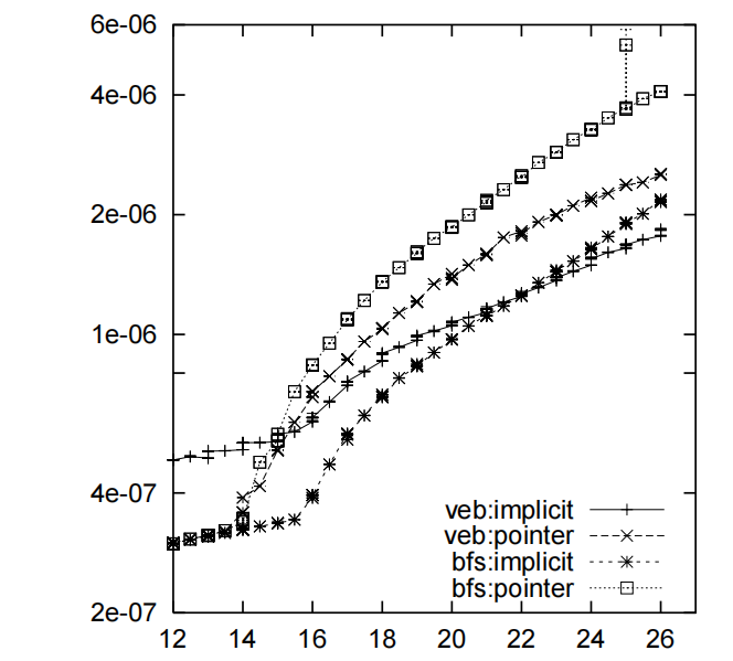
Figure 8. Performance of pointer-based vs. array-based implementations of vEB and BFS
From the first experiment above, we draw a preliminary conclusion: vEB and BFS are worth studying further, while the other two layouts don’t perform very well. So next, the authors directly compare the vEB and BFS layouts side by side
in their pointer-based and array-based implementations.
BFS: the implicit version always beats the pointer version, which shows that “computing addresses” is no slower than “following pointers”.
vEB: within the cache the pointer version is faster, but outside the cache the implicit version turns the tables. The reason is that without pointers, the same block can hold more nodes (B gets larger).
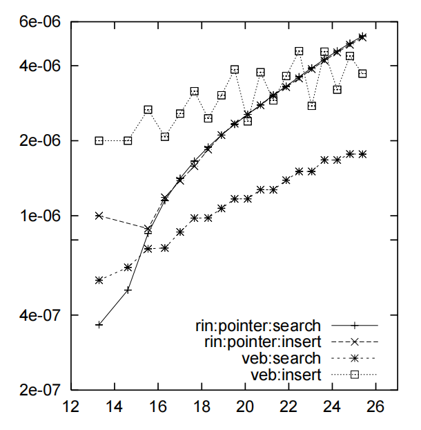
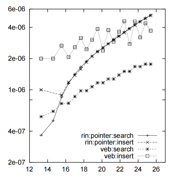
Figure 9. vEB vs. an unbalanced tree: insertion and search performance
From Fig 9 we can roughly draw the following conclusion: if the system is mostly doing searches with only occasional updates (updates here meaning inserts), the semi-dynamic vEB is better around n≈216 (the lowest curve).
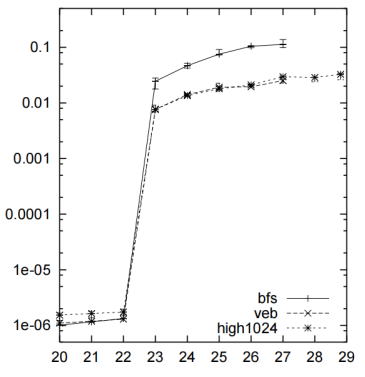
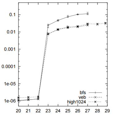
Figure 10. Performance comparison beyond main memory
Within main memory, BFS is the fastest; once the size of main memory is exceeded, BFS instead becomes more than 5× slower (note that the vertical axis in the figure is not linear). The 1024-ary tree optimized for the page size is the fastest outside main memory,
but about 2× slower within main memory (again, the vertical axis is not linear). vEB, by contrast, keeps pace with the best of the structures all the way, performing stably across levels.
Authors’ conclusions
The memory hierarchy dominates running time, even when the tree is still far smaller than main memory.
The benefits of cache-obliviousness hold in practice: vEB is competitive with cache-aware schemes, almost always better than “unoptimized” schemes, and robust across multiple memory levels.
The space savings / larger fan-out (larger B) brought by the implicit (pointer-free) layout contribute significantly to performance; the dynamic scheme is both easy to implement and shows good time performance.
5. Reflection
The implicit, cache-oblivious search tree of small height achieves the B-tree’s lower bound on I/O performance, laying a solid foundation for robust range queries across the board.
With the vEB layout, its I/O cost can be kept at O(logBn+Bk),
and these optimality results still hold in 2025; however, the “backbone” could also be replaced by other structures (such as the cache-oblivious B-Tree).
Given the steadily increasing capacity of hardware at every level (registers, L1/L2/L3 caches, main memory), as well as modern techniques such as prefetching, branch prediction, and SIMD,
other approaches are often faster than this paper’s scheme in some purely in-memory scenarios; we will discuss potential improvements later.
For root-to-leaf accesses, the vEB layout has a clean logBn complexity (the formula here appears garbled in the original),
and it usually outperforms other schemes when n≥threshold. Compared with prior work, the small-height tree does not need weight balancing,
avoiding heavy or frequent updates; instead, it redistributes the tree only when necessary. Note that when n≤threshold
(the original formula is likewise garbled), the implicit array-based layout incurs extra overhead because index computation becomes the dominant cost; as n grows,
this overhead turns into a trade-off against pointer chasing. The array-based layout also means that the effective capacity n of a single transferred block is larger, so one I/O can fetch more data.
A rebuild of the whole tree (H←H+1) is triggered only when n grows enough that the root violates the rule; consecutive rebuilds are separated by Θ(n) updates, so the cost amortized over each update is small.
Having summarized the strengths, we should also look at the shortcomings. As Fig 9 shows,
although the vEB layout performs better in the large-scale insertion comparison, its performance jitters fairly often, which in the long run may affect the overall behavior of the hardware and the system.
In addition, it is clear that the vEB scheme performs well at larger cache scales but falls behind other schemes with smaller caches.
The caches and memory of modern CPUs keep growing, which to some extent limits its potential range of application.
Modern I/O models typically involve multi-level caches (L1/L2/L3), the page cache, and the NVMe protocol.
The two-level I/O model used in this paper is fairly idealized: it only analyzes block transfers between two levels and ignores factors beyond the cache line, such as the TLB and page size—something already reflected in the
Cache-Conscious B+ Tree.
Furthermore, this paper mainly discusses the data structure in a single-threaded context, whereas modern systems commonly use multi-threaded access and care more about latch-free or incremental updates
to reduce the cache invalidation and lock contention caused by shared writes; the Bw-Tree discusses this specifically.
Finally, it’s worth emphasizing that the cache-oblivious B-tree proposed in 2005 retains this paper’s core advantages—fast lookups and range scans across all levels of the memory hierarchy—
while not requiring periodic subtree rebuilds. It is easier to operate, friendlier to concurrent reads and writes, and works well everywhere from CPU caches to SSDs without manual tuning;
it stays compact, with low pointer overhead and strong locality, while also delivering smoother performance and lower engineering cost.
Reference
Footnotes
P. van Emde Boas. Preserving order in a forest in less than logarithmic time and linear space. Inf. Process. Lett., 6:80–82, 1977. ↩
H. Prokop. Cache-oblivious algorithms. Master’s thesis, Massachusetts Institute of Technology, June 1999. ↩
S. Chatterjee, V. V. Jain, A. R. Lebeck, S. Mundhra, and M. Thottethodi. Nonlinear array layouts for hierarchical memory systems. In Proceedingsof the 1999 Conference on Supercomputing, ACM SIGARCH, pages 444–453.ACM Press, 1999. ↩