Pre-requirement

# general preparation
python -m pip install -U pip setuptools wheel
python -m pip install -U pybind11 numpy
sudo apt install -y build-essential
 
# install package
python setup.py install
 
# run the test script
python main.py

My environment information:

OS: WSL2
CPU: Intel Core i7-13700H
- L1d: 480 KiB (10 instances)
- L1i: 320 KiB (10 instances)
- L2: 12.5 MiB (10 instances)
- L3: 24 MiB (1 instance)
Memory: 16GB

Cache-oblivious GEMM Implementation Report

To implement and see what’s the difference between the different method, I decided to set up the environment as C++ implementation and python invokation as well as benchmarking. So we need to install pybind11 and numpy and matplotlib before our experiment.

The data type we choose for this experiment is float32.

To be aware of different optimizations’ effect on GEMM, I decided to arrange and extend this report in a step-by-step order, which is also a common and straight-forward way followed by all high-performance computing programmer.

v1: naive GEMM

The very first thing is to implement a naive version, with nearly no optimization:

#define OFFSET(i, j, ld) ((i * ld) + j)
 
// single precision gemm, float32
void sgemm_naive(float* a, float* b, float* c, const size_t M, const size_t N, const size_t K) {
    for (int i = 0; i < M; i++) {
        for (int j = 0; j < N; j++) {
            for (int k = 0; k < K; k++) {
                c[OFFSET(i, j, N)] += a[OFFSET(i, k, K)] * b[OFFSET(k, j, N)];
            }
        }
    }
}

Our testing matrix sizes ranges from 32 to 1024, (from $2^5$ to $2^{10}$ ), 6 groups in total.

To benchmark the performance, we need to adopt the standarized symbol: GFLOPS to measure our program, this is a metric we would have seen in multiple libraries of high performance computing.

The total float operation of GEMM could be computed as: $FLOPs \approx 2 \times M \times N \times K$ , and GFLOPS could also be computed as:

GFLOPS = \frac{FLOPS}{10^9 \times runtime}

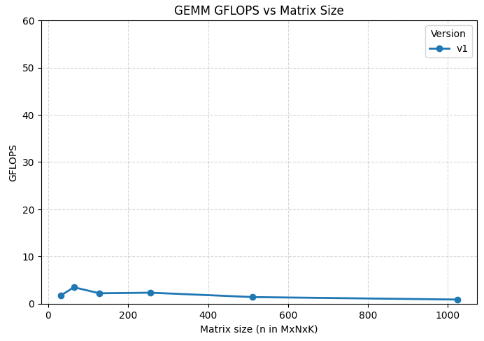
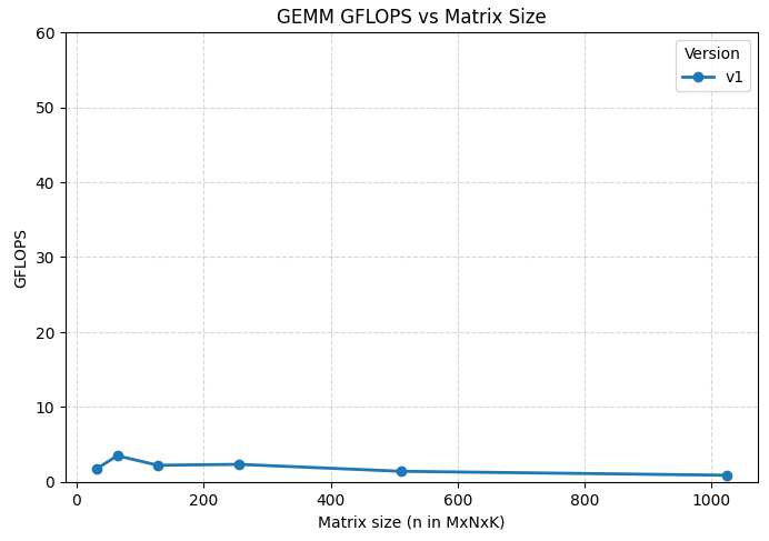
Based on this simple and efficient metric setting, we could easily draw a figure like this:

It’s pretty plain, and as I have expected and observed in the past CPU GEMM implementations. The naive GEMM implementation got 2.90 GFLOPS at best case when $MNK=64$ . As I could infer, this could be the best size for trading off the matrix block size, and the cache size.

Note in advance that, the reason why the y-axis was set at range of 0 to 60 is that, I used to implement a certain version of cache-aware GEMM, and reached the GFLOPS=55.8, so I knew that 60 would be the maximum value.

v2: Strategy: Multi-Threading

Maybe this strategy is applied too early, but I still prefer to adopt this optimization at the very first time.

The reason why using multi-threading strategy could be listed as follows:

Each thread is only responsible for one block of result matrix $C$ . For a 512 x 512 matrix, assuming we have 8 threads, each thread would compute a 128 x 256 block of $C$ , and all 8 threads compute 8 blocks, which will finally compose a complete matrix. What is the most important is that, threads could compute in parallel, which reduces the runtime.
When it comes to cache, (L1, L2 cache), it is owned by physical CPU core. By applying multi-thread strategy, we bind each thread to a CPU core, which is making best use of its own cache, as well as setting up a good environment for us to optimize the cache access pattern in the later part. So I choose to apply this strategy first.

There is one concern, that modern CPUs are built with SMT technique, which means one physical CPU core could handle two simultaneous threads, if we have 8 CPU cores, should we launch 16 threads?

My previous CPU-GEMM optimization experience proved that, it would be better to keep the same amount of threads as physical CPU cores, the reason is that, although two threads could compute in parallel, they could also compete for the L1 and L2 cache space, too. In order to avoid such “cache race”, keeping it simple could be the better choice.

V2 code could be as follow:

template <const int NUM_THREADS = 8 /* The device may have more than 8 cores, but to align with matrix size, use 8 cores to compte*/>
void sgemm_v2(float* a, float* b, float* c, const size_t M, const size_t N, const size_t K) {
    // use multi thread to handle this GEMM process
    const int TILE_SIZE_X = M / (NUM_THREADS / 2);  // ------------ > x, the horizon
    const int TILE_SIZE_Y = N / (2);                // y, the vertical
    #pragma omp parallel num_threads(NUM_THREADS)
    {
        const int total_threads = omp_get_num_threads();
        const int tid = omp_get_thread_num();       // current tid, same programming model as cuda
        const int tile_id_x = tid % (NUM_THREADS / 2);
        const int tile_id_y = tid / (NUM_THREADS / 2);
        const int block_x = tile_id_x * TILE_SIZE_X;
        const int block_y = tile_id_y * TILE_SIZE_Y;
 
        // compute
        for (int m = 0; m < TILE_SIZE_Y; m++) {
            int start_idx_m = block_y + m;
            for (int n = 0; n < TILE_SIZE_X; n++) {
                int start_idx_n = block_x + n;
                for (int k = 0; k < M; k++) {
                    c[OFFSET(start_idx_m, start_idx_n, N)] += a[OFFSET(start_idx_m, k, K)] * b[OFFSET(k, start_idx_n, N)];
                }
            }
        }
    }
}

Here I chose to use OpenMP as the parallel computation library, because launching threads manually will lead to extra overhead, comparing to use one highly-optimized library. Meanwhile, to keep code clean and simple, as well as focusing on the topic cache-oblivious GEMM, I would like to save the strength on such code style discussion.

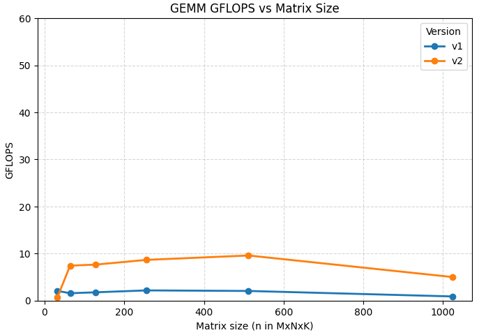
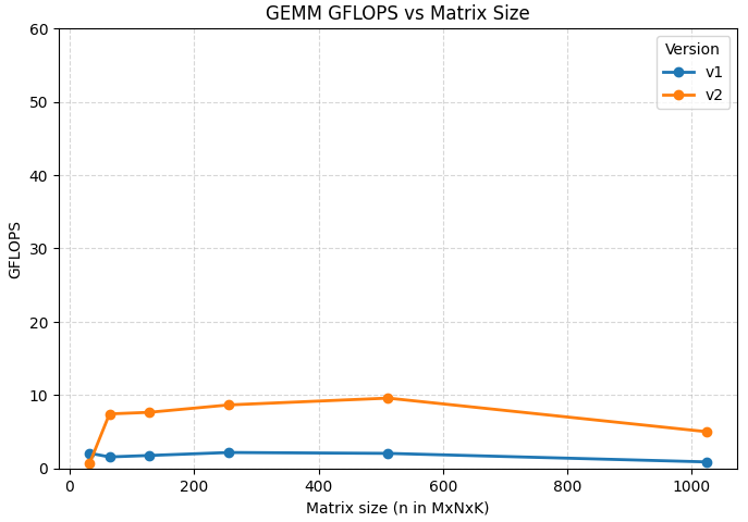
Each thread will compute its starting index of matrix block, and computes in parallel, the benchmark:

The highest GFLOPS is 9.58 at $MNK=512$ , then drops to 5.00 at $MNK=1024$ , the speedup compared to naive group is nearly $5\times$ , except the first group. I think that when MNK size is small, the multi-thread’s launching and collecting cost would dominate the process, thus v2 is slower than v1 at $MNK=32$ .

v3: Scheme: Recursive Divide

The title starts with scheme, instead of strategy, because our requirement is to implement a recursive divide and conquer GEMM. So this step is to meet the basic requirement, not an optimization attempt.

Now we will discuss how to implement a cache-oblivious GEMM. My attempt is to divide the matrix into 4 blocks each time, recursively, untill the block size is less than a certain threshold.

Assuming the matrix size is 512 x 512, after our threading strategy, each thread would compute a 256 x 128 block. This is the start point for our recursive division applying. For a 256 x 128 block, define a threshold size 64, the divide steps could be described as follows:

1st division, 256 x 128 → [128 x 64] x 4
2st division, 128 x 64 → [64 x 32] x 4

Now both $M$ and $N$ have been limited to our setting threshold, we would develop a micro kernel, to compute a small block’s GEMM.

Note that, there are a lot of variables to be created for computing the index, which is confused and puzzling. To avoid this I would like to clarify here:

C_M, C_N, C_K is the abbreviation of current M, current N, current K size, [64, 32] e.g.
lda, ldb, ldc is the leading dimension of matrix. Although we are computing a tiny block, in order to get the correct index we will fetch data across rows and columns, thus leading dimension should be clarified, and distinguished from current matrix size. 512 e.g.
global_start_x, global_start_y is the global coordination of our starting point, as we have mentioned that we are doing multi-thread computation, each thread would have a starting point to figure out the exact location.

Considering the tight textual space of this report, I will not represent the total v3 code, but I would present only the recursive method:

// the input a,b,c will be added the thread block offset before passing in.
template <const int TILE_SIZE = 64>
void sgemm_v3_recursive(float* a, float* b, float* c, 
                            size_t C_M, size_t C_N, size_t C_K, 
                            size_t lda, size_t ldb, size_t ldc) {
    if (C_M <= TILE_SIZE && C_N <= TILE_SIZE) {
        sgemm_v3_micro_kernel(a, b, c, C_M, C_N, C_K, lda, ldb, ldc);
        return;
    }
 
    // divide recursively
    // assume we divide the matrix 2x2
    const size_t M_u = C_M / 2;     // `u` stands for up
    const size_t M_d = C_M - M_u;   // `d` stands for down
    const size_t N_l = C_N / 2;     // `l` stands for left
    const size_t N_r = C_N - N_l;
 
    sgemm_v3_recursive(a,               b,              c,                      M_u, N_l, C_K, lda, ldb, ldc);
    sgemm_v3_recursive(a + M_u * lda, b,            c + M_u * ldc,          M_d, N_l, C_K, lda, ldb, ldc);
    sgemm_v3_recursive(a,               b + N_l,    c + N_l,                M_u, N_r, C_K, lda, ldb, ldc);
    sgemm_v3_recursive(a + M_u * lda, b + N_l,      c + M_u * ldc + N_l, M_d, N_r, C_K, lda, ldb, ldc);
}

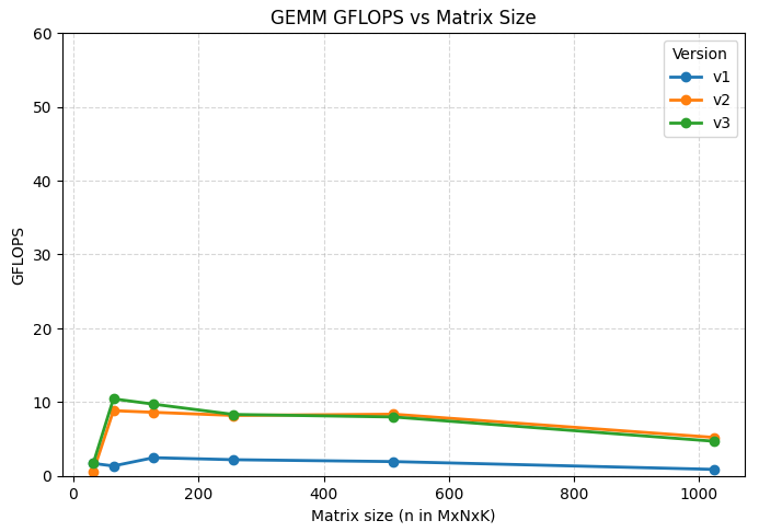
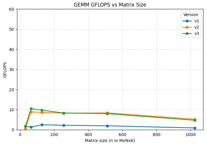
Each level divide the matrix block to 4 smaller blocks, recursively, the benchmark:

Obviously, the result did not meet our expectation. A smaller block size will lead to better and more friendly cache access pattern, boosting performance improvement, but the result we observed contradicts with this prior experience.

To address this issue, let’s review the potential improvement points:

Why the recursive way is 2 x 2? Any existing previous research demonstrates that this is the best recursive way?
Why the threshold is 64? Any existing blogs or paper demonstrates this value’s effectiveness?
Why inner product? The outer product could be better.
Although we have divided the blocks, we only divide the result matrix $C$ , that is to say, our computation way of smallest matrix block could also be described as:
1. ```
a block: [tile_size, total_K] @ b block: [total_K, tile_size] = c block: [tile_size, tile_size]
 
e.g.
a block: [64, 512] @ b block: [512, 64] = c block: [64, 64]
```
2. which means: I am still accessing the long-wide total range, not matter in a, b or c, which strongly against our initial intention of recursive GEMM.
3. Alternatively, I should find a way that only computes one small block each time, like a [8x8] @ [8x8], instead of computing the whole range.

v4: Strategy: Accelerate the divide pattern

After sorting out all potential ways, I decided to improve the cache-oblivious recursive GEMM from following aspects:

The division strategy: the previous division is rough, and only divides $C$ into blocks, in order to reach the real small-block GEMM, I modified the division logic:

template <const int BASE = 64 /* threshold */>
void sgemm_v4_recursive(
    const float* __restrict A,
    const float* __restrict B,
    float* __restrict       C,
    size_t C_M, size_t C_N, size_t C_K,
    size_t lda, size_t ldb, size_t ldc)
{
    if (C_M <= (size_t)BASE && C_N <= (size_t)BASE && C_K <= (size_t)BASE) {
        sgemm_micro_v4_blockbuffer_kernel<BASE>(A, B, C, C_M, C_N, C_K, lda, ldb, ldc);
        return;
    }
 
    // split recursively along the longest dim
    if (C_M >= C_N && C_M >= C_K) {
        // split M
        const size_t M1 = C_M / 2;
        const size_t M2 = C_M - M1;
        sgemm_v4_recursive<BASE>(A,              B, C,              M1, C_N, C_K, lda, ldb, ldc);
        sgemm_v4_recursive<BASE>(A + M1 * lda,   B, C + M1 * ldc,   M2, C_N, C_K, lda, ldb, ldc);
    } else if (C_N >= C_M && C_N >= C_K) {
        // split N
        const size_t N1 = C_N / 2;
        const size_t N2 = C_N - N1;
        sgemm_v4_recursive<BASE>(A, B,             C,             C_M, N1, C_K, lda, ldb, ldc);
        sgemm_v4_recursive<BASE>(A, B + N1,        C + N1,        C_M, N2, C_K, lda, ldb, ldc);
    } else {
        // split K: this is outer product!
        const size_t K1 = C_K / 2;
        const size_t K2 = C_K - K1;
        sgemm_v4_recursive<BASE>(A,           B,             C, C_M, C_N, K1, lda, ldb, ldc);
        sgemm_v4_recursive<BASE>(A + K1,      B + K1 * ldb,  C, C_M, C_N, K2, lda, ldb, ldc);
    }
}

At this time, we split $A, B$ and $C$ matrix into smaller blocks, and operates real small-block GEMM, to make our GEMM cache harmonious.
Meanwhile, our recursively splitting strategy is half-largest-split, each time we will split the largest dimension to two halves. This strategy ensures that we could get a pretty-resized small matrix block, instead of getting some long-ranged sub-matrix.

Kernel Optimization: Our kernel is still a naive one, no buffering, cross row accessing, etc. I decided to optimize our kernel in following aspects:
1. Accessing A, B, and C matrix block in row, instead of cross-row accessing. This will keep data linear in cache, and accessing them continuously. Of course this requires some re-order of computating method.
2. Re-order the triple loop. As we all know, GEMM requires at least three loop: i,j,k, but the order of them could be re-arranged. In previous implementation I just used i, j, k, but how about i,k,j or k,i,j? I tried to find the best combination of this triple loop sequence.
3. Buffering. C[i,j] += A[i,k] * B[k,j] is naive and plain. To be more specific, this would cause one read and one write from cache each time. What about we use some variables as buffer, sum, e.g. This variable is stored in registers instead of cache or memory, which is the fastest. After finishing adding, write it back to C[i,j], saving a lot of reading overhead.

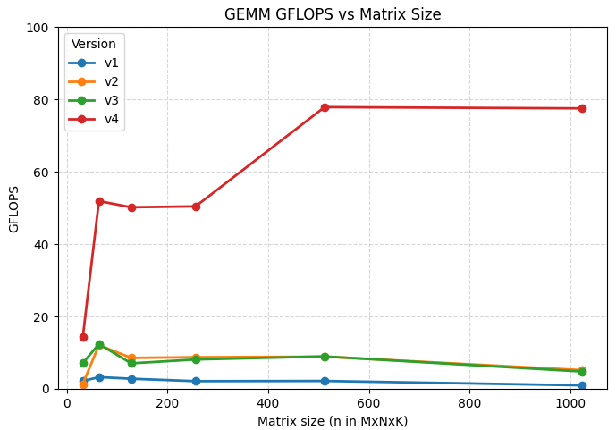
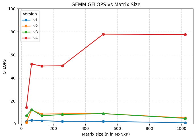
It’s astonishing. I break the record of my previous best implementation’s GFLOPS (55.8, 1 year ago). The highest GFLOPS at $MNK=1024$ is 77.55!

There are still some factors I need to consider:

Why $MNK=64$ GFLOPS is so high? And drops down in $MNK=256,512$ ? This remains a mystery.
The TILE_SIZE I used is 64, what about tuning this size?
The kernel is not fully optimized yet (AVX2 Instruction Set) , which means our program still has optimizing space.

v4-plus: Tune: Experiment on `TILE_SIZE`

Before tuning the TILE_SIZE, I would like to put my reflection on the correctness of this approach.

Core issue: What we are doing is implementing a cache-oblivious recursive GEMM. Note that, it’s cache-oblivious. If we tune the TILE_SIZE, will this action contradict to our initial intention?

No, they do not contradict to each other. Indeed we are doing cache-oblivious things, and the function does not know the exact cache-size, but the function urgently needs to know when to stop, instead of endless recursion. Besides, the TILE_SIZE would significantly affect our micro-kernel’s performace, we need to do experiments to see which size would boost our micro-kernel most.

Based on such debating and reflection, let’s tune the TILE_SIZE in [16, 32, 48, 64, 96, 128]. This requires some C++ dispatch to invoke different template tile_base, which would be detailed in code implementation, not be presented in report context.

Different TILE_SIZEs are experimented as follows:

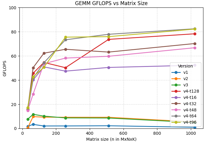
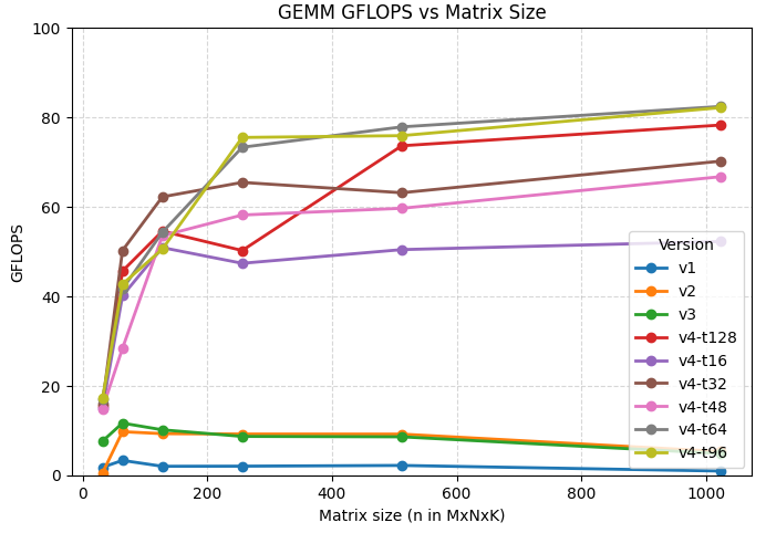
As shown in this figure, best performance was reached when TILE_BASE=64, and group-t64, group-t96 could nearly perform the same at large GEMM. As for small GEMM like $MNK=64,128$ , the TILE_SIZE would significantly affect the performance among which the group-t128 has best performance. The peak GFLOPS is 79.71 by group-t64 at $MNK=1024$ .

In the rest optimization steps, I will use the best performance group TILE_SIZE = 64 to test the hardware limit, as we have tested out that this size could have best performance.

v5: Strategy: AVX2

We haven’t apply avx2 instruction set to our program yet. Let’s do this to our micro-kernel, which is pretty easy.

The avx2 implementation is plain, which could be regarded as “a translation of previous micro-kernel to 4-element continuous” versoin. The code will not be expanded in report, benchmark:

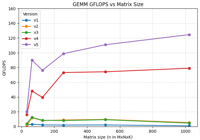
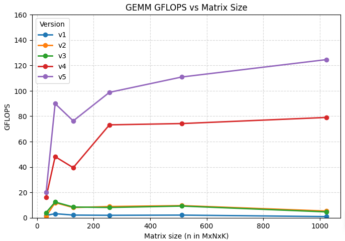
The peak GFLOPS at $MNK=1024$ is 108.83, almost $1.36 \times$ speed up compared to v4, this improvement does not meet our expectation. SIMD instructions operates 4-float-element fmadd each time. Considering the memory access, computation, and other potential affected parts, the speedup would be at least $2\times$ .

In another word, current implementation performed very poorly.

Again, let’s review the potential optimization in our micro-kernel:

Our current computing scheme is inner product, according to modern BLAS libraries, outer product could be better.
According to technique blogs or public discussion¹, 8x6 tile size could be a better (or even best) tiny-tile for SIMD. I have known this trick, but I haven’t implemented any version yet. Let’s try at this time.
1. Note that: This typical tile-size requires the matrices are col-major
We are currently depending on for loop, this actually did a lot of thing for us, and jumped a lot of optimization chances. We need to unroll this loop manually, instead of using #pragma unroll

v6: Strategy: AVX2 - Enhanced version

In this section, I applied all my previous optimization strategy:

Converting $A, B$ to col-major, for outer-production.
Inside micro-kernel, doing small 8x6 tile size GEMM, the total size of this micro-kernel is 64x64, thus applying padding at the tail part.
Unroll the loop manually, to make sure variables stay in register/L1 cache/L2 cache.
Buffering.

Detailed implementation is a bit large, thus would not be presented in our report.

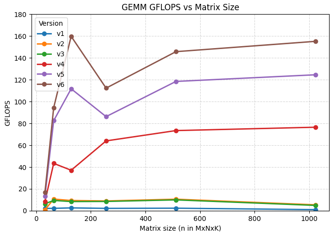
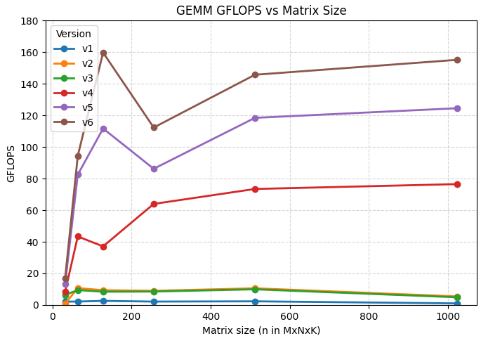
In comparison, the GFLOPS peak at $MNK=1024$ by v6 is $151.28$ , while v5 is $119.37$ , and v4 is $80.75$ , which means v6 (highly-optimized AVX2 version) has almost $2\times$ speedup compared to v4 (No AVX2 versoin).

So far, I have tried all optimization strategies I could have known and learned.

Although I have also known that doing data-repacking would help boost the performance further more, I think these are all enough.

v7: Strategy: Packing

Data packing is a strategy to arrange micro-kernel’s all accessing data in advance, storing them in a buffer, and reuse them in a linear memory access manner, instead of fetching them from L2 cache / memory.

We need to be aware that: the packing is not part of GEMM itself, it’s optional and not compulsory, which will introduce extra overhead. So the question is: can overhead of data-packing trade off with the performance boosting it brings? Let’s implement and checkout:

    // packing A
    alignas(32) float Apack[BASE * 8];
    for (int k = 0; k < (int)C_K; ++k) {
        const float* ap = A + (size_t)k * lda + i0; // A[i0:i0+8, k]
        __m256 avec = (im == 8) ? _mm256_loadu_ps(ap)
                                : _mm256_maskload_ps(ap, rmask);
        _mm256_store_ps(Apack + k * 8, avec);
    }
 
    for (size_t j0 = 0; j0 < C_N; j0 += 6) {
        const int jm = (int)std::min<size_t>(6, C_N - j0);
 
        // packing B: transpose
        alignas(32) float Bpack[BASE * 8];
        int bp_ofs = 0;
        for (int kb = 0; kb < (int)C_K; kb += 8) {
            const int u = std::min(8, (int)C_K - kb);
            const __m256i kmask = (u == 8) ? _mm256_set1_epi32(-1) : mask8(u);
            for (int t = 0; t < jm; ++t) {
                const float* src = B + (size_t)(j0 + t) * ldb + kb; // B[kb:kb+u, col]
                __m256 v = (u == 8) ? _mm256_loadu_ps(src)
                                    : _mm256_maskload_ps(src, kmask);
                _mm256_store_ps(Bpack + bp_ofs + t*8, v);
            }
            bp_ofs += 6 * 8; // next 6*8 tile
        }
        
        // ....
        
    }

Benchmark:

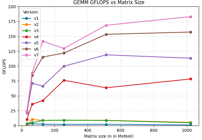
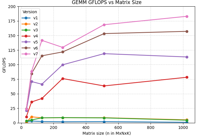
After packing, the v7 reached $GFLOPS=182.95$ at peak. And v4 is $78.19$ , which means v7 (highly-optimized AVX2 version) has $2.33 \times$ speedup compared to v4 (No AVX2 version). And this observation answers the question: The extra overhead that packing data brings, would eventually trade off with performance boosting that it leads to.

Conclusion & Reflection

This is quite an unforgettable journey. Throughout this journey I got another chance to implement CPU GEMM on hand by myself again, and I got deeper unstanding on cache-oblivous method and reviewed my past implementations. In this section I would conclude our optimization strategies and answer several questions.

We have applied: multi-threading, recursive-divide-and-conquer, re-arranging divide pattern, tuning TILE_SIZE, using AVX2 and doing very radical optimization to AVX2 kernel, improving GFLOPS from $0.88$ to $182.95$ , which is offensively approaching the limit of our hardware. The most importantly, I beat the past myself, as well as the performance I used to reach.

The biggest advance, surprisingly, does not come from any my previous known strategies, but from v3: recursive divide to v4: accelerate the divide pattern (from the last figure, from $4.76$ to $80.44$ , boosting $16.89 \times$ speedup). The latter strategies were just help improving, but never made such a break-through, which proves the effectiveness of cache-oblivious implementation and the correctness of cache-oblivious theory, again.

Now I would like to reflect on several specific questions:

1. Why 8x6 would be the best tile size?

The word best I used in my report, is a little bit rushed. Only under the scenarios of float32 - AVX2 - col-major - outer-product GEMM, 8x6 could be a perfect tile size. To prove it, I would like to compute this process directly.

In col-major layout of matrix, we often adopt outer-product GEMM pattern to be hardware-friendly.
In outerr product, we take one col from left matrix A [M, 1]. and one row from right matrix B [1, N], to do computation, thus forming a result matrix of [M, N], and then add to result matrix $C$ .
At the same time, due to the col-major layout:
- “one col from A” actually means a row, in physical layout of A.
- “one row from B” actually means a col, in physical layout of B.
AVX2-256bit, could exactly store 8 float32 elements in a __m256 data.
- which means, a __m256 data could be stored in a ymm register. (Perfectly suit-in)
- So, we could store one physical row of A.
Each time, we broadcast a scalar of B, to __m256, and do _mfadd256() with previous A data.
- Note: we do not load a linear fragment of B, but broadcast a single one scalar of B instead.
Lastly, add the result to “one col of C”, and “one col” also means a row, in physical layout of C.

Let’s consider the registers usage in this 8x6 trick:

ymm0-ymm5 → store “6 cols of C”, with 8 elements each. That is the size of 8x6.
ymm6 → store the temp variable of “one col of A”, one __m256 data only takes one register.
ymm7 → store the temp variable of “broadcasted scalar of B”, one __m256 data only takes one register.

So, a 8x6 small tile takes 8 ymm registers in total. Although one CPU core has 16 ymm registers, the rest ymm registers would be used for other purposes, such as bufferring, data-transferring, etc. Any attempt to allocate more ymm registers would lead to performance dropping.

Beyond registers, the cache line could also be considered. Modern CPU’s cache line is 64B. The usage of 8 ymm registers take $8\times256\;bits = 8 \times 8 \; B = 64\;B$ , perfectly making good use of one cache line.

2. Why performance boosts at $MNK=64, 128$ ? And why it drops steeply later then?

Again, we could compute this GEMM total size:

$64 \times 64 \times 4 \;B= 16KB$ , $A+B+C=48KB$ . My working CPU has exactly 48KB L1d Cache per CPU core, which means the whole GEMM operation could landing mostly in L1 Cache.
$128 \times 128 \times 4\;B = 64KB$ , $A+B+C = 192KB$ . Altough this would over-flow my L1 data cache, it could still land most in L2 Cache.

Based on this observatoin, it seems explainable for the temporary peak.

Starting from $M=N=K=256$ , $256 \times 256 \times 4\;B = 256 KB$ , $A+B+C=768KB$ , which exceeds the L2 cache size. The reuse of cache would be in a bad situation, and even worse if we are not doing re-packing of data. This could explain the steep dropping in the figure.

Reference

Why 8x6 tile size is better: https://github.com/bluss/matrixmultiply/issues/34#issue-386834699 ↩

Pre-requirement

# general preparation
python -m pip install -U pip setuptools wheel
python -m pip install -U pybind11 numpy
sudo apt install -y build-essential
 
# install package
python setup.py install
 
# run the test script
python main.py

My environment information:

OS: WSL2
CPU: Intel Core i7-13700H
- L1d: 480 KiB (10 instances)
- L1i: 320 KiB (10 instances)
- L2: 12.5 MiB (10 instances)
- L3: 24 MiB (1 instance)
Memory: 16GB

Cache-oblivious GEMM Implementation Report

The data type we choose for this experiment is float32.

v1: naive GEMM

The very first thing is to implement a naive version, with nearly no optimization:

#define OFFSET(i, j, ld) ((i * ld) + j)
 
// single precision gemm, float32
void sgemm_naive(float* a, float* b, float* c, const size_t M, const size_t N, const size_t K) {
    for (int i = 0; i < M; i++) {
        for (int j = 0; j < N; j++) {
            for (int k = 0; k < K; k++) {
                c[OFFSET(i, j, N)] += a[OFFSET(i, k, K)] * b[OFFSET(k, j, N)];
            }
        }
    }
}

Our testing matrix sizes ranges from 32 to 1024, (from $2^5$ to $2^{10}$ ), 6 groups in total.

To benchmark the performance, we need to adopt the standarized symbol: GFLOPS to measure our program, this is a metric we would have seen in multiple libraries of high performance computing.

The total float operation of GEMM could be computed as: $FLOPs \approx 2 \times M \times N \times K$ , and GFLOPS could also be computed as:

GFLOPS = \frac{FLOPS}{10^9 \times runtime}

Based on this simple and efficient metric setting, we could easily draw a figure like this:

Note in advance that, the reason why the y-axis was set at range of 0 to 60 is that, I used to implement a certain version of cache-aware GEMM, and reached the GFLOPS=55.8, so I knew that 60 would be the maximum value.

v2: Strategy: Multi-Threading

Maybe this strategy is applied too early, but I still prefer to adopt this optimization at the very first time.

The reason why using multi-threading strategy could be listed as follows:

Each thread is only responsible for one block of result matrix $C$ . For a 512 x 512 matrix, assuming we have 8 threads, each thread would compute a 128 x 256 block of $C$ , and all 8 threads compute 8 blocks, which will finally compose a complete matrix. What is the most important is that, threads could compute in parallel, which reduces the runtime.
When it comes to cache, (L1, L2 cache), it is owned by physical CPU core. By applying multi-thread strategy, we bind each thread to a CPU core, which is making best use of its own cache, as well as setting up a good environment for us to optimize the cache access pattern in the later part. So I choose to apply this strategy first.

There is one concern, that modern CPUs are built with SMT technique, which means one physical CPU core could handle two simultaneous threads, if we have 8 CPU cores, should we launch 16 threads?

V2 code could be as follow:

template <const int NUM_THREADS = 8 /* The device may have more than 8 cores, but to align with matrix size, use 8 cores to compte*/>
void sgemm_v2(float* a, float* b, float* c, const size_t M, const size_t N, const size_t K) {
    // use multi thread to handle this GEMM process
    const int TILE_SIZE_X = M / (NUM_THREADS / 2);  // ------------ > x, the horizon
    const int TILE_SIZE_Y = N / (2);                // y, the vertical
    #pragma omp parallel num_threads(NUM_THREADS)
    {
        const int total_threads = omp_get_num_threads();
        const int tid = omp_get_thread_num();       // current tid, same programming model as cuda
        const int tile_id_x = tid % (NUM_THREADS / 2);
        const int tile_id_y = tid / (NUM_THREADS / 2);
        const int block_x = tile_id_x * TILE_SIZE_X;
        const int block_y = tile_id_y * TILE_SIZE_Y;
 
        // compute
        for (int m = 0; m < TILE_SIZE_Y; m++) {
            int start_idx_m = block_y + m;
            for (int n = 0; n < TILE_SIZE_X; n++) {
                int start_idx_n = block_x + n;
                for (int k = 0; k < M; k++) {
                    c[OFFSET(start_idx_m, start_idx_n, N)] += a[OFFSET(start_idx_m, k, K)] * b[OFFSET(k, start_idx_n, N)];
                }
            }
        }
    }
}

Each thread will compute its starting index of matrix block, and computes in parallel, the benchmark:

v3: Scheme: Recursive Divide

Now we will discuss how to implement a cache-oblivious GEMM. My attempt is to divide the matrix into 4 blocks each time, recursively, untill the block size is less than a certain threshold.

1st division, 256 x 128 → [128 x 64] x 4
2st division, 128 x 64 → [64 x 32] x 4

Now both $M$ and $N$ have been limited to our setting threshold, we would develop a micro kernel, to compute a small block’s GEMM.

Note that, there are a lot of variables to be created for computing the index, which is confused and puzzling. To avoid this I would like to clarify here:

C_M, C_N, C_K is the abbreviation of current M, current N, current K size, [64, 32] e.g.
lda, ldb, ldc is the leading dimension of matrix. Although we are computing a tiny block, in order to get the correct index we will fetch data across rows and columns, thus leading dimension should be clarified, and distinguished from current matrix size. 512 e.g.
global_start_x, global_start_y is the global coordination of our starting point, as we have mentioned that we are doing multi-thread computation, each thread would have a starting point to figure out the exact location.

Considering the tight textual space of this report, I will not represent the total v3 code, but I would present only the recursive method:

// the input a,b,c will be added the thread block offset before passing in.
template <const int TILE_SIZE = 64>
void sgemm_v3_recursive(float* a, float* b, float* c, 
                            size_t C_M, size_t C_N, size_t C_K, 
                            size_t lda, size_t ldb, size_t ldc) {
    if (C_M <= TILE_SIZE && C_N <= TILE_SIZE) {
        sgemm_v3_micro_kernel(a, b, c, C_M, C_N, C_K, lda, ldb, ldc);
        return;
    }
 
    // divide recursively
    // assume we divide the matrix 2x2
    const size_t M_u = C_M / 2;     // `u` stands for up
    const size_t M_d = C_M - M_u;   // `d` stands for down
    const size_t N_l = C_N / 2;     // `l` stands for left
    const size_t N_r = C_N - N_l;
 
    sgemm_v3_recursive(a,               b,              c,                      M_u, N_l, C_K, lda, ldb, ldc);
    sgemm_v3_recursive(a + M_u * lda, b,            c + M_u * ldc,          M_d, N_l, C_K, lda, ldb, ldc);
    sgemm_v3_recursive(a,               b + N_l,    c + N_l,                M_u, N_r, C_K, lda, ldb, ldc);
    sgemm_v3_recursive(a + M_u * lda, b + N_l,      c + M_u * ldc + N_l, M_d, N_r, C_K, lda, ldb, ldc);
}

Each level divide the matrix block to 4 smaller blocks, recursively, the benchmark:

To address this issue, let’s review the potential improvement points:

Why the recursive way is 2 x 2? Any existing previous research demonstrates that this is the best recursive way?
Why the threshold is 64? Any existing blogs or paper demonstrates this value’s effectiveness?
Why inner product? The outer product could be better.
Although we have divided the blocks, we only divide the result matrix $C$ , that is to say, our computation way of smallest matrix block could also be described as:
1. ```
a block: [tile_size, total_K] @ b block: [total_K, tile_size] = c block: [tile_size, tile_size]
 
e.g.
a block: [64, 512] @ b block: [512, 64] = c block: [64, 64]
```
2. which means: I am still accessing the long-wide total range, not matter in a, b or c, which strongly against our initial intention of recursive GEMM.
3. Alternatively, I should find a way that only computes one small block each time, like a [8x8] @ [8x8], instead of computing the whole range.

v4: Strategy: Accelerate the divide pattern

After sorting out all potential ways, I decided to improve the cache-oblivious recursive GEMM from following aspects:

The division strategy: the previous division is rough, and only divides $C$ into blocks, in order to reach the real small-block GEMM, I modified the division logic:

template <const int BASE = 64 /* threshold */>
void sgemm_v4_recursive(
    const float* __restrict A,
    const float* __restrict B,
    float* __restrict       C,
    size_t C_M, size_t C_N, size_t C_K,
    size_t lda, size_t ldb, size_t ldc)
{
    if (C_M <= (size_t)BASE && C_N <= (size_t)BASE && C_K <= (size_t)BASE) {
        sgemm_micro_v4_blockbuffer_kernel<BASE>(A, B, C, C_M, C_N, C_K, lda, ldb, ldc);
        return;
    }
 
    // split recursively along the longest dim
    if (C_M >= C_N && C_M >= C_K) {
        // split M
        const size_t M1 = C_M / 2;
        const size_t M2 = C_M - M1;
        sgemm_v4_recursive<BASE>(A,              B, C,              M1, C_N, C_K, lda, ldb, ldc);
        sgemm_v4_recursive<BASE>(A + M1 * lda,   B, C + M1 * ldc,   M2, C_N, C_K, lda, ldb, ldc);
    } else if (C_N >= C_M && C_N >= C_K) {
        // split N
        const size_t N1 = C_N / 2;
        const size_t N2 = C_N - N1;
        sgemm_v4_recursive<BASE>(A, B,             C,             C_M, N1, C_K, lda, ldb, ldc);
        sgemm_v4_recursive<BASE>(A, B + N1,        C + N1,        C_M, N2, C_K, lda, ldb, ldc);
    } else {
        // split K: this is outer product!
        const size_t K1 = C_K / 2;
        const size_t K2 = C_K - K1;
        sgemm_v4_recursive<BASE>(A,           B,             C, C_M, C_N, K1, lda, ldb, ldc);
        sgemm_v4_recursive<BASE>(A + K1,      B + K1 * ldb,  C, C_M, C_N, K2, lda, ldb, ldc);
    }
}

At this time, we split $A, B$ and $C$ matrix into smaller blocks, and operates real small-block GEMM, to make our GEMM cache harmonious.
Meanwhile, our recursively splitting strategy is half-largest-split, each time we will split the largest dimension to two halves. This strategy ensures that we could get a pretty-resized small matrix block, instead of getting some long-ranged sub-matrix.

Kernel Optimization: Our kernel is still a naive one, no buffering, cross row accessing, etc. I decided to optimize our kernel in following aspects:
1. Accessing A, B, and C matrix block in row, instead of cross-row accessing. This will keep data linear in cache, and accessing them continuously. Of course this requires some re-order of computating method.
2. Re-order the triple loop. As we all know, GEMM requires at least three loop: i,j,k, but the order of them could be re-arranged. In previous implementation I just used i, j, k, but how about i,k,j or k,i,j? I tried to find the best combination of this triple loop sequence.
3. Buffering. C[i,j] += A[i,k] * B[k,j] is naive and plain. To be more specific, this would cause one read and one write from cache each time. What about we use some variables as buffer, sum, e.g. This variable is stored in registers instead of cache or memory, which is the fastest. After finishing adding, write it back to C[i,j], saving a lot of reading overhead.

It’s astonishing. I break the record of my previous best implementation’s GFLOPS (55.8, 1 year ago). The highest GFLOPS at $MNK=1024$ is 77.55!

There are still some factors I need to consider:

Why $MNK=64$ GFLOPS is so high? And drops down in $MNK=256,512$ ? This remains a mystery.
The TILE_SIZE I used is 64, what about tuning this size?
The kernel is not fully optimized yet (AVX2 Instruction Set) , which means our program still has optimizing space.

v4-plus: Tune: Experiment on `TILE_SIZE`

Before tuning the TILE_SIZE, I would like to put my reflection on the correctness of this approach.

Different TILE_SIZEs are experimented as follows:

In the rest optimization steps, I will use the best performance group TILE_SIZE = 64 to test the hardware limit, as we have tested out that this size could have best performance.

v5: Strategy: AVX2

We haven’t apply avx2 instruction set to our program yet. Let’s do this to our micro-kernel, which is pretty easy.

The avx2 implementation is plain, which could be regarded as “a translation of previous micro-kernel to 4-element continuous” versoin. The code will not be expanded in report, benchmark:

In another word, current implementation performed very poorly.

Again, let’s review the potential optimization in our micro-kernel:

Our current computing scheme is inner product, according to modern BLAS libraries, outer product could be better.
According to technique blogs or public discussion¹, 8x6 tile size could be a better (or even best) tiny-tile for SIMD. I have known this trick, but I haven’t implemented any version yet. Let’s try at this time.
1. Note that: This typical tile-size requires the matrices are col-major
We are currently depending on for loop, this actually did a lot of thing for us, and jumped a lot of optimization chances. We need to unroll this loop manually, instead of using #pragma unroll

v6: Strategy: AVX2 - Enhanced version

In this section, I applied all my previous optimization strategy:

Converting $A, B$ to col-major, for outer-production.
Inside micro-kernel, doing small 8x6 tile size GEMM, the total size of this micro-kernel is 64x64, thus applying padding at the tail part.
Unroll the loop manually, to make sure variables stay in register/L1 cache/L2 cache.
Buffering.

Detailed implementation is a bit large, thus would not be presented in our report.

So far, I have tried all optimization strategies I could have known and learned.

Although I have also known that doing data-repacking would help boost the performance further more, I think these are all enough.

v7: Strategy: Packing

    // packing A
    alignas(32) float Apack[BASE * 8];
    for (int k = 0; k < (int)C_K; ++k) {
        const float* ap = A + (size_t)k * lda + i0; // A[i0:i0+8, k]
        __m256 avec = (im == 8) ? _mm256_loadu_ps(ap)
                                : _mm256_maskload_ps(ap, rmask);
        _mm256_store_ps(Apack + k * 8, avec);
    }
 
    for (size_t j0 = 0; j0 < C_N; j0 += 6) {
        const int jm = (int)std::min<size_t>(6, C_N - j0);
 
        // packing B: transpose
        alignas(32) float Bpack[BASE * 8];
        int bp_ofs = 0;
        for (int kb = 0; kb < (int)C_K; kb += 8) {
            const int u = std::min(8, (int)C_K - kb);
            const __m256i kmask = (u == 8) ? _mm256_set1_epi32(-1) : mask8(u);
            for (int t = 0; t < jm; ++t) {
                const float* src = B + (size_t)(j0 + t) * ldb + kb; // B[kb:kb+u, col]
                __m256 v = (u == 8) ? _mm256_loadu_ps(src)
                                    : _mm256_maskload_ps(src, kmask);
                _mm256_store_ps(Bpack + bp_ofs + t*8, v);
            }
            bp_ofs += 6 * 8; // next 6*8 tile
        }
        
        // ....
        
    }

Benchmark:

Conclusion & Reflection

Now I would like to reflect on several specific questions:

1. Why 8x6 would be the best tile size?

In col-major layout of matrix, we often adopt outer-product GEMM pattern to be hardware-friendly.
In outerr product, we take one col from left matrix A [M, 1]. and one row from right matrix B [1, N], to do computation, thus forming a result matrix of [M, N], and then add to result matrix $C$ .
At the same time, due to the col-major layout:
- “one col from A” actually means a row, in physical layout of A.
- “one row from B” actually means a col, in physical layout of B.
AVX2-256bit, could exactly store 8 float32 elements in a __m256 data.
- which means, a __m256 data could be stored in a ymm register. (Perfectly suit-in)
- So, we could store one physical row of A.
Each time, we broadcast a scalar of B, to __m256, and do _mfadd256() with previous A data.
- Note: we do not load a linear fragment of B, but broadcast a single one scalar of B instead.
Lastly, add the result to “one col of C”, and “one col” also means a row, in physical layout of C.

Let’s consider the registers usage in this 8x6 trick:

ymm0-ymm5 → store “6 cols of C”, with 8 elements each. That is the size of 8x6.
ymm6 → store the temp variable of “one col of A”, one __m256 data only takes one register.
ymm7 → store the temp variable of “broadcasted scalar of B”, one __m256 data only takes one register.

2. Why performance boosts at $MNK=64, 128$ ? And why it drops steeply later then?

Again, we could compute this GEMM total size:

$64 \times 64 \times 4 \;B= 16KB$ , $A+B+C=48KB$ . My working CPU has exactly 48KB L1d Cache per CPU core, which means the whole GEMM operation could landing mostly in L1 Cache.
$128 \times 128 \times 4\;B = 64KB$ , $A+B+C = 192KB$ . Altough this would over-flow my L1 data cache, it could still land most in L2 Cache.

Based on this observatoin, it seems explainable for the temporary peak.

Reference

Why 8x6 tile size is better: https://github.com/bluss/matrixmultiply/issues/34#issue-386834699 ↩

Cache Oblivious GEMM Implementation

Cache Oblivious GEMM Implementation

Pre-requirement

Cache-oblivious GEMM Implementation Report

v1: naive GEMM

v2: Strategy: Multi-Threading

v3: Scheme: Recursive Divide

v4: Strategy: Accelerate the divide pattern

v4-plus: Tune: Experiment on `TILE_SIZE`

v5: Strategy: AVX2

v6: Strategy: AVX2 - Enhanced version

v7: Strategy: Packing

Conclusion & Reflection

Reference

Pre-requirement

Cache-oblivious GEMM Implementation Report

v1: naive GEMM

v2: Strategy: Multi-Threading

v3: Scheme: Recursive Divide

v4: Strategy: Accelerate the divide pattern

v4-plus: Tune: Experiment on `TILE_SIZE`

v5: Strategy: AVX2

v6: Strategy: AVX2 - Enhanced version

v7: Strategy: Packing

Conclusion & Reflection

Reference

Pre-requirement

Cache-oblivious GEMM Implementation Report

v1: naive GEMM

v2: Strategy: Multi-Threading

v3: Scheme: Recursive Divide

v4: Strategy: Accelerate the divide pattern

v4-plus: Tune: Experiment on TILE_SIZE

v5: Strategy: AVX2

v6: Strategy: AVX2 - Enhanced version

v7: Strategy: Packing

Conclusion & Reflection

Reference

Footnotes

Pre-requirement

Cache-oblivious GEMM Implementation Report

v1: naive GEMM

v2: Strategy: Multi-Threading

v3: Scheme: Recursive Divide

v4: Strategy: Accelerate the divide pattern

v4-plus: Tune: Experiment on TILE_SIZE

v5: Strategy: AVX2

v6: Strategy: AVX2 - Enhanced version

v7: Strategy: Packing

Conclusion & Reflection

Reference

Footnotes

v4-plus: Tune: Experiment on `TILE_SIZE`

v4-plus: Tune: Experiment on `TILE_SIZE`