Ever since I first got into HPC a long time ago, I had heard of flash attention1. Later, during my research internship, flash attention v22 had just come out, but back then I simply used it via pip install, and when I saw the formulas and illustrations in the paper, I didn’t dig too deeply. Later still, during my internship at Paddle, an opportunity came up: my leader asked me to compare the quantized operator I had reproduced against flash attention v33 to see which one was stronger. So I came into contact with the v3 operator, but because of a tight task schedule, it was once again just pip install, and I still didn’t go and understand the principles behind it.
To stop being a pip install boy, and since I happen to have some time right now to settle down and build up my inner strength, I decided to read through flash attention from v1 to v3 and organize it into a document for future reference. At the same time, I’ve recently been stuck at a bottleneck in kernel development: it feels like I know everything, and yet also like I know nothing. So why not look at how people think about data and kernels, and how they make use of the latest features, in textbook-level practice — the unity of knowledge and action.
Admittedly, there are already many existing write-ups on flash attention. Although few of them tie everything together into one thread, by reading them together and merging them, you can always piece together a complete line of knowledge. Inspired by DefTruth’s article4, I settled on the order for studying and organizing: online softmax → FA1 → FA2 → FA3.
2. Prerequisite: Softmax[all]
2.1 Safe Softmax
The formal expression of the attention computation shows where the softmax function is used. In practice, because the softmax operation is memory-bound during inference, many researchers have proposed ways to optimize this formula.
The most naive formula for softmax is: softmax(xi)=∑j=1Nexjexi. Typically, in an implementation we do a warp-block reduce to obtain a sum, and then perform the element-wise softmax operation.
The engineering problem with the original softmax is that, when training or running inference in fp16, the exponent xi can be very large, so exi overflows easily. To put a quantitative estimate on it: fp16 can represent values up to the order of 65536, and once xi≥11, exi already overflows 65536. Under these circumstances, the concept of safe softmax was proposed. (By the way, here’s a link to a clean implementation of safe softmax)
Safe Softmax can be expressed as:
∑j=1Nexjexi→∑j=1Nexj−mexi−m
Every exponent has m subtracted from it, where m is the maximum over all xi: m=max(xi). The purpose of this is to guarantee that the exponent ends up less than 0, which in effect greatly reduces the risk of numerical overflow.
2.2 Online Softmax
In fact, suppose we implement this version of softmax on a CPU (more formally: in an ordinary programming model rather than SIMT); we’ll find that it takes at least 3 passes to complete:
In the first for loop, find the maximum value in the set xi, denoted m
In the second for loop, accumulate to finally compute a sum, i.e., the ∑j=1Nexj−m part, which serves as the denominator
In the third for loop, divide each element one by one by the denominator computed in the second step, and write the results back to the output space
Now let’s look at how to do the computation online5.
In the scheme above, the three for loops cannot be fused with one another, because they have sequential dependencies: the second step depends on the first step finding the global maximum m, and the third step depends on the second step computing the global sum. If we want to push the complexity as low as possible and reduce accesses to global memory, the only option is to hack the formula ourselves — find an online method that is nearly equivalent to the original formula.
The approach proposed by online softmax is to replace m, the global maximum, with the “current maximum” mi: the maximum over the region scanned so far is used as m. This process can be formally expressed as:
(Since this article emphasizes connecting the dots, I simply included the earlier formulas as well, so you can get an intuitive feel for how the formula evolves.)
At this point, we can pull out the denominator and analyze it on its own. Let dS=∑j=1Sexj−mS, where S denotes the index we’ve computed up to so far; it evolves as follows:
dS=j=1∑Sexj−mS=j=1∑S−1exj−1−mS+exj−mS
This step simply pulls the last term out on its own.
With this, we have completed the derivation of the recurrence, linking each dS to dS−1.
What’s the use of this step? The point is: of the three loops above, we can fuse the first and second steps, so softmax can now be computed with only two for loops.
In the first for loop, compute the running maximum mS scanned so far (just compare it directly with mS−1); and, alongside it, compute the sum up to the current position.
In the second for loop, perform the element-wise division by the total sum computed
OK, let’s set online softmax aside for now as prerequisite knowledge; next, we move on to reading flash attention v1.
3. Flash Attention-v1
Flash Attention v1 (hereafter FA-v1) aims to provide a general-purpose operator for all GPU devices, so it can’t present its content primarily from the NVIDIA GPU perspective; hence it uses the two terms HBM and SRAM. HBM is short for GPU high bandwidth memory; its counterpart on NVIDIA GPUs is what we usually call global memory. SRAM is the umbrella term for all on-chip memory; this set includes {′shared_memory′,′registers′,′caches′} and so on, not just shared memory. So a distinction and clarification is needed here; there’s a discussion6 on the NVIDIA forums about this.
FA-v1’s optimizations mainly target the I/O pattern of the attention computation, making targeted use of SRAM. It also extends Flash Attention to a block-sparse attention computation, which is faster than all existing attention acceleration methods (FA-v1 was proposed in 2022).
At that time, linear attention7 had not yet been proposed, and the complexity of attention still grew quadratically with the sequence length (denoted N), i.e., N2. Existing acceleration schemes did all reduce the complexity of attention as much as possible through various approximation methods, but they mostly focused on theoretical FLOP reductions, which did not match the observed actual running time (called wall-clock speedup in the paper), and these works tended to ignore the overhead of memory access.
We’ll skip the background for now and assume everyone has some GPU & CUDA & HPC fundamentals; this article only covers the optimization ideas and contributions of FA-v1 through v3.
3.1 Engineering Model of Standard Attention
When computing attention, we usually deal with tensor shapes like [bsz, n_head, seq_len, head_dim], where the last two dims, sequence length and head dimension, are formally denoted N and d respectively. FA-v1 summarizes the attn computation with the following formulas:
S=QKT∈RN×N,P=softmax(S)∈RN×N,O=PV∈RN×d
In general, seq_len is far larger than head_dim. For example, we often talk about long sequences of length 32K, while the model’s head_dim is only 128; here 32×1024>>128, i.e., N>>d. So this process is actually IO-dominated and memory-bound. The paper presents the standard attention computation as pseudocode; here I’ll lay it out in plain words:
Load Q,K from global memory into each thread’s private local memory or register (the threads evenly share the elements of QK), do one GEMM S=QKT, then write the result S back to global memory.
Then fetch S from global memory, compute P=softmax(S), and write the result P back to global memory
Load P,V from global memory again, do the GEMM O=PV, then write O back to global memory
Output O
After reading this part, I wonder whether FA-v1’s way of modeling attention is a bit too plain; in reality, anyone who knows even a little HPC wouldn’t design a kernel like this. Going in and out of global memory three times is far too expensive. If this really is how everyone computed attention before FA-v1 came out, it must have been painful.
FA-v1 sets its core goal: reduce accesses to global memory. The ideal would be to load from global memory once, finish the entire computation, and then write back to global memory. Although it doesn’t ultimately achieve such an idealized single read and single write, it still drastically reduces the number of global memory accesses compared with the original setup.
To achieve this goal, FA-v1 mainly proposes two techniques: Tiling and Recomputation.
3.2 The Concept of Tiling in FA-v1
Before going further, I’d like to first sort out the various notions of tiling I’ve encountered since getting into HPC, to avoid confusion.
What is a tile — the most basic definition
When we do kernel optimization, the basic programming model (the CUDA Programming Guide) tells you that our programming model is grid-block-thread. The PTX programming model tells you that our programming model is CTA-cluster-grid. The concept of a tile comes up when the data partitioning scheme goes below the block size, and it is adopted for cache-locality friendliness, or register friendliness. For example, if a block’s data is 256×256, it will be split into small 8×8 or 16×16 tiles before being submitted for computation.
A tile is a minimal unit of data partitioning, and also an optimization strategy; it isn’t part of the programming model in any official programming guide.
If I had to pick a keyword, I’d use slice strategy instead
The tile in PTX
Friends who have worked with SM90 and above, or who have read the PTX documentation firsthand, should know that in low-level PTX instructions, fixed-size data blocks such as .m16n16k16 and .m32n8k16 are also called tiles. In this context, the tile effectively becomes a specific hardware specification prescribed for programming; it is more a term for instruction-level fragment shape / register fragment layout, which determines the fragment mapping and instruction throughput, and doesn’t directly carry the program-level semantics of “putting data into shared/register and how to pipeline it”. When we use mma or wmma, we always keep an eye on how the data is partitioned so that it fits these sizes, and arrange our own kernel logic accordingly.
If I had to pick a keyword, I’d use fragment size instead
The tile in tile-lang
I’ve been following tile-lang8 for a while (a really excellent repository). It’s a domain-specific-language compiler developed based on the ideas of TVM9, in which the tile is elevated to a first-class citizen: in tile-lang, a tile is both a data-partitioning concept and a program abstraction and scheduling unit.
If I had to pick a keyword, I’d use scheduling unit instead
Back to the main topic: the tile in flash attention
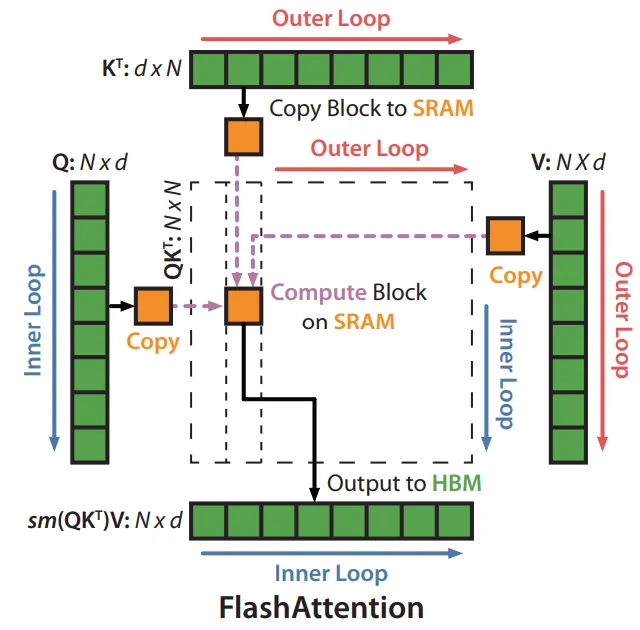
In FA-v1, loading all of Q,K,V into shared memory at once is clearly unrealistic. The best approach is to split them into small blocks one after another; formally, the small orange blocks can be denoted Qblock,Kblock,Vblock. During computation, we only need to load these small blocks into shared memory and finally compute Oblock; before adding it back to its corresponding position, we scale Oblock by the right normalization factor and then add it back, which yields the correct result.
Applying softmax to dQKT is a tricky problem. Although we already have the online softmax method, the situation now is: the matrix to be softmaxed has seq_len rows and head_dim columns, and softmax must be applied to each row. If we did softmax row by row, we’d have to run online softmax seq_len times. Even though we’ve now partitioned into blocks, we still need to run online softmax over each small block.
Prior work10 has already proposed an optimization: suppose there are only two rows in total, [2, head_dim]; each row can be pulled out on its own as a vector, denoted x(1),x(2) in the paper. Combining this with the earlier online softmax formula while ensuring numerical stability, the paper proposes the following computation:
m(x)=m([x(1)x(2)])here this denotes the concat of the two vectors=max(m(x(1)),m(x(2)))f(x)=[em(x(1))−m(x)f(x(1))em(x(2))−m(x)f(x(2))]
Here, f(x) denotes the concat of the numerator parts of the two elements after online softmax has been computed on each.
Actually, the formulas here are not stated very clearly in places; if you find them obscure, please refer to the original paper1 and DefTruth’s blog4.
A few questions immediately arise:
How do we partition QKV? As we all know, during attention computation QKV have two dimensions, [seq_len, head_dim]; which dimension do we split along? How large should each piece be?
How do we compute with Qblock,Kblock,Vblock?
Partition size and pseudocode walkthrough
In the HPC field, when memory access is involved, it’s customary to use B for block size and M for memory size; this convention was already in use in research from many years ago (cache-aware, cache-oblivious), and FA-v1 is no exception. For each sequence, for each attention head during the computation, we can formalize as follows:
Q,K,V∈RN×d, the total size of shared memory is M
The block sizes are set to: Bc=⌈4dM⌉, Br=min(⌈4dM⌉,d)
This answers the first question: how big a chunk to cut KV into. From the formula: 4dM is the size of the K/V column blocks. Each time we process, we need to put such K and V column blocks (note: column-major!) into shared mem. Why this size? Let’s do a quick calculation, assuming fp16 inference:
One block occupies: Bc×d×2bytes
K and V each have one block, occupying in total: 2×Bc×d×2bytes=4Bcdbytes
Assuming our shared memory size is M, to guarantee no overflow we need Bc≤4dM. In practice, based on my hands-on experience using Flash Attention before, after rounding up, Bc is usually 16 or 32, to fit the mma.m?n?k? PTX instructions.
And how big a chunk do we cut Q into? min(⌈4dM⌉,d). We’ll explain later why it’s this size; for now, let’s continue describing FA-v1’s computation process:
Initialize on HBM the O matrix of size N×d; the sum vector l(x) of size N; and the vector m(x) that temporarily stores the maxima, of size N.
Split Q along the seq_len dimension (this answers the first question: which dimension to split along), each block of size Br, yielding Tr=⌈BrN⌉ blocks in total: Q1,Q2,...,QTr, each of size Br×d (i.e., the data of Br tokens x head_dim)
Split K,V along the seq_len dimension (note, however, that seq_len is a column vector in KV, so what we actually get is a column block), yielding Tc=⌈BcN⌉ blocks in total: K1,K2,...,KTc, V1,V2,...,VTc, each of size Bc×d (i.e., the data of Bc tokens x head_dim)
Split O in the same way as Q, obtaining O1,O2,O3,...,OTr, each of size Br×d.
Split the two vectors l,m; here the original paper uses the phrase divideintoblocks, obtaining l1,l2,..,lTr and m1,m2,...,mTr, each of size Br
Personally, I find this not quite accurate: they are row vectors to begin with, and blocks sounds like a 2D matrix; in reality, it’s just slicing arrays. Calling it divideintoslices might be a bit easier to understand.
Now that we’ve sorted out the data partitioning logic, let’s move on to the computation logic:
Outer loop (clearly marked in orange in the figure, mainly used to advance the KV blocks): load KV blocks from global memory into shared memory
Inner loop (marked in blue in the figure, mainly used to advance the Q and O blocks): load the corresponding Qi,Oi blocks from global memory into shared memory;
Compute the attention score in shared memory: Sij=QiKiT∈RBr×Bc
Compute in shared memory mij=rowmax(Sij)∈RBr, Pij=eSij−mij∈RBr×Bc, lij=rowsum(Pij)∈RBr
Compute minew,linew in shared memory; this is where these vectors are dynamically maintained
The scaling factor we mentioned earlier: diag(linew)−1(diag(li)emi−minewOi+emij−minewPijVj); once computed, write it back to Oi‘s corresponding position in global memory
Write the newly maintained linew,minew back to global memory
end inner loop
end outer loop
3.3 Recomputation
We have indeed adopted the approach of splitting along the seq_len dimension. The next question that immediately arises is: if we want to store P=softmax(S), then as the sequence grows we’d eventually need an estimated O(N2) of GPU memory, along with an enormous accompanying cost of memory reads and writes (I/O overhead). Our block-wise reading approach is nice — discard the current block once it’s computed — but if we want to get the output O=PV in one go, we usually need to keep quite a few intermediate variables in shared memory.
One of Flash Attention’s goals is to make all the intermediate data that needs to be stored as small as possible, ideally compressing it down to the order of O(N). The idea is to trade expensive I/O for doing a bit more computation (note: grasping the idea is what matters most; these ideas and experiences help us write more efficient kernels during development). This is clearly reasonable, because on GPU devices computation is simply cheaper than IO; this way, we can also improve the wall-clock speed somewhat.
The steps of recomputation can be formalized as follows:
Split the task into two scans over the c-blocks: the first only computes the normalization factors, and the second multiplies the weights by V:
Pass-1: for each c-block:
mt=max(x(t)),ℓt=∑ex(t)−mt; merge them with the global (m,ℓ) using the online formula.
Afterwards, we only need to store m,ℓ for each row, both on the order of O(N) in size; there’s no need to store S,P
Pass-2: directly compute the normalized weights:
ω(t)=ℓex(t)−m
Multiply by V: r←r+ω(t)V(t)
After scanning all blocks, output Oi=r
3.4 I/O Analysis
I’ll skip the proofs here; interested readers can head straight to the paper. Here we just record the conclusions.
The IO complexity of standard attention is: Θ(Nd+N2), where d is head_dim
The IO complexity of Flash-Attention is: Θ(MN2d2), where M is the size of shared memory. This directly explains FA-v1’s advantage: the reduction in IO is what determines the speedup.
We won’t go into “block-sparse FlashAttention” here, since it isn’t part of the main thread; interested readers can explore it on their own.
4. Flash Attention-v2
FA-v1’s performance reaches only 25-40% of the theoretical peak FLOPS. The reason behind this is the lack of a partitioning strategy sufficiently optimized across blocks, threads, and warps, which results in low occupancy and unnecessary shared memory reads/writes. Note that this sentence is a highly condensed, distilled one from the abstract; in the analysis below, we’ll make clear what exactly went wrong and what optimizations were made.
FA-v2 is mainly developed on the A100. To optimize to the extreme, you first need to know the A100’s hardware parameters, so that we can understand where the hardware’s limits lie.
The A100 has 81GB of GPU memory (global memory) with 1.5−2.0TB/s of bandwidth, a total of 192KB of shared memory, 108 SMs, and 19TB/s of on-chip bandwidth. Since the L2 cache can’t be controlled programmatically, the paper still centers its optimization efforts on global memory and shared memory.
For FA-v1, we expanded on lots of formulas and discussed the concrete steps of kernel optimization. Starting from FA-v2, the walkthrough will mainly record the ideas: with the groundwork laid earlier, discussing the optimization schemes goes more smoothly, and you won’t be left unable to form a mental picture. But the rest of the article won’t be as detailed as the introduction to Flash Attention-v1.
This is also what the great DefTruth advised in his article: be meticulous when going through FA-v1, mainly in order to master the principles.
Therefore, for the subsequent FA-v2 and FA-v3, we focus on presenting the optimization ideas.
4.1 Improving the Algorithm to Save Space
Viewed from FA-v2’s perspective, the computational approach of the earlier FA-v1 algorithm still needs to keep too much in shared memory, and it also has some extra computation steps. FA-v2 made the following optimizations:
Going from O(2)=diag(ℓ(2)ℓ(1))−1O(1)+diag(ℓ(2))−1eS(2)−m(2)V(2) to O~(2)=diag(ℓ(1))−1O(1)+eS(2)−m(2)V(2). Note that in the new formula, O~(2) is un-scaled data, so we only need to scale the last O~(last) once by diag(ℓ(last))−1 at the end of the loop to obtain the final output.
At the same time, we no longer need to store both m(j),ℓ(j) for the backward pass; instead, storing a single variable L(j)=m(j)+log(ℓ(j)) (logsumexp) is enough.
With these two changes, we save both computation steps and shared memory space.
Handling the causal mask
Attention inference always requires a causal mask, i.e., a lower-triangular matrix. Since FA-v1 already cut the sequence into a grid of row blocks r and column blocks c, for any row r and column c:
If c>r, i.e., the entire block lies in the upper triangle, skip it directly.
This way, for a long sequence, half of the blocks can be skipped, which in theory directly cuts the amount of computation by 2×; taking into account fixed overheads such as data loading, synchronization, and pipelining, the measured speedup is 1.7−1.8×.
Meanwhile, for the “diagonal blocks”, element-wise masking is applied, i.e.: per-row only 1 block masked.
For c<r, the entire block lies in the lower triangle; compute it normally
For c>r, skip it
For c=r, i.e., the diagonal block, this block does have some data in the upper triangle and some in the lower triangle; we only need to apply an element-wise causal mask inside this block, setting all positions with j>i within the block to −∞. This way, each row only needs masking in 1 block, and every other block is either fully computed or fully skipped, which avoids a lot of branching and also eliminates some pipeline bubbles.
4.2 Changing the Parallelization Strategy
In FA-v1, parallelism is applied over two dimensions: batch-size and num_head. We use 1 cuda block to compute one attention head of one sequence, which means a total of bsz×n_heads cuda blocks are launched. If each block runs on one SM — say the device we’re using is an A100 with 108 SMs in total — this scheduling scheme is reasonably efficient when batch_size is very large, e.g., batch_size > 80. But when the batch size is relatively small and seq_len is very long, or when num_heads is small (GQA), this parallelization strategy isn’t that efficient.
This time, to solve this problem during inference, it was decided to also make the seq_len dimension a dimension of parallel computation. In other words, after the same sequence is split into different blocks, the blocks are submitted directly to different cuda-blocks (i.e., distributed to different SMs) for computation, since this process doesn’t require them to pass information to one another; meanwhile, parallelism over the batch_size and num_head dimensions is retained as well. This way, whether it’s a large batch, large or small num_head, or long or short sequences, the kernel is guaranteed to run in its most efficient form, making the most of the GPU’s hardware throughput.
This design is implemented mainly by swapping the order of the loops inside the kernel: the outer-loop covers row-blocks, and the inner-loop covers col-blocks.
4.3 Changing How Data Is Partitioned Across Warps
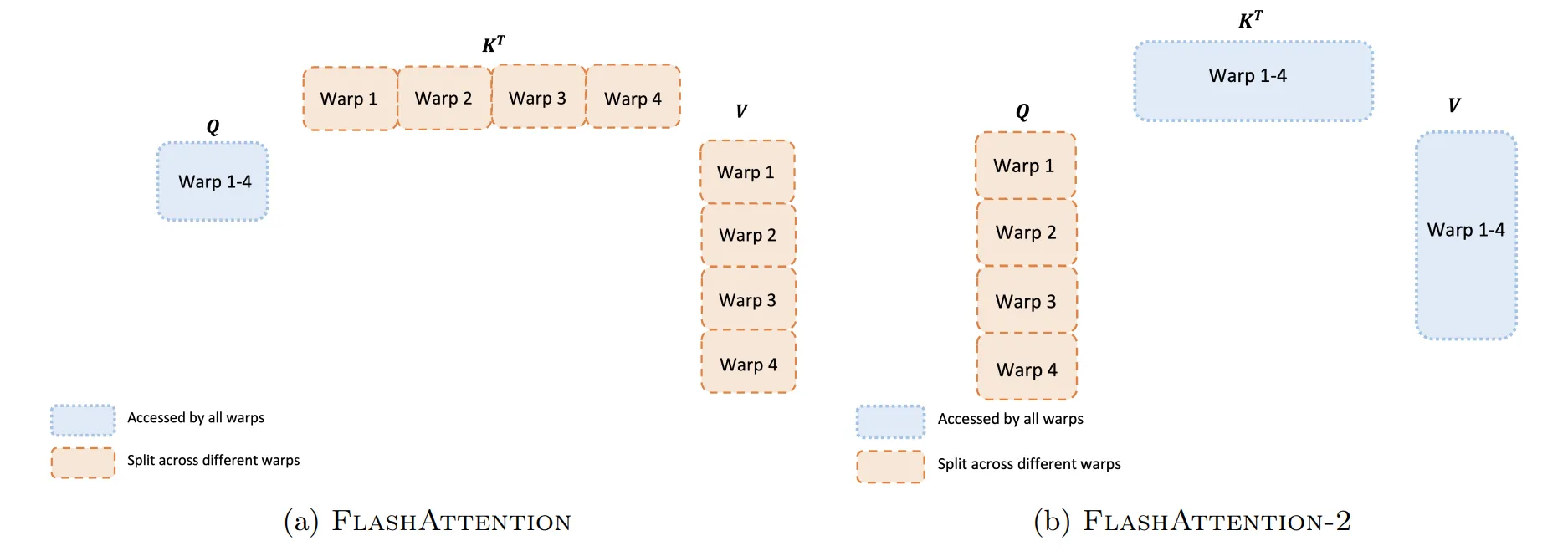
The way warps access data in FA-v1 is shown on the left. Warps 1-4 can all access the Q-block, while for K and V, each warp fetches its own portion of the data and then performs the QKV computation. As a result, each warp is responsible for computing a QKT and also for computing with its corresponding Vslice, and in the end communication between the different warps is required to add everything up and form the result. The paper calls this the “Split-K” scheme.
What makes this scheme inefficient is that all warps need to store their results into shared memory, synchronize (perhaps via __syncthreads()), and finally sum. The heavy shared memory reads/writes, along with the synchronization they require, are FA-v1’s pain point, and FA-v2 sets out to eliminate this step entirely.
The way warps access data in FA-v2 is shown on the right. Warps 1-4 are each responsible for fetching one slice of Q, and this time KV becomes data that warps 1-4 can all access. This is called the “split-Q” scheme.
This way, each slice only needs to compute its own QKT and then multiply by V to get the corresponding output, with no cross-warp communication needed. Naturally, this doesn’t involve much shared memory reading/writing and also saves the synchronization cost, so it directly speeds things up.
At this point, FA-v2’s optimization methods have been roughly covered. Note that the backward-pass content hasn’t been gone through in much detail; interested readers please head straight to the original paper.
5. Flash Attention-v3
As its abstract also mentions, FA-v3 was proposed precisely because FA-v2 performed too poorly on the H100, with GPU utilization of only 35%.
FA-v3, I believe, is also a well-worn topic for most people: it optimizes by exploiting the asynchronous features for tensor cores and the native .tensor data type[^11] available starting with SM90, the TMA feature, and FP-8 mixed-precision inference support. The concrete results are as follows:
It reaches 740 TFLOPS with FP16 inference, i.e., 75% H100 utilization.
FP8 inference reaches 1.2 PFLOPS.
The FP8 inference accuracy in FA-v3 is 2.6× better than the baseline FP8 Attention results.
5.1 Introduction
For the H100 GPU, the programming model has changed a lot. Before going further, let’s do a brief overview here. This overview comes not only from the paper but also from my own prior experience, presented to everyone in what I hope is the easiest-to-understand way:
Note: the H100 is an SM90-arch GPU
On GPUs before SM90, the mainstream GPU programming model was still grid-block-thread: kernels are launched onto SMs in units of blocks, and shared memory is private to an SM, shared by all threads running within that SM. Shared memory can’t be shared across SMs.
On GPUs at SM90 and above, optimization has gone deep down to the PTX level. The PTX programming model, from top to bottom, is: grid-cluster-CTA[^12], where a CTA can be understood as equivalent to the block concept in our earlier programming model. A group of CTAs forms a cluster, and shared memory can be shared at the cluster level; that is, a group of SMs now forms a cluster, and that group of SMs can share shared memory.
TMA, a term everyone keeps bringing up, is actually a dedicated hardware unit on Hopper-architecture GPUs, mainly used for data movement; it can perform asynchronous copies of data from global memory to shared memory.
.tensor is a native data type in PTX programming. Indeed, on devices below SM90 and at or above SM80, you can use the cp.async instruction, but there’s a catch: it can only move ordinary data, not .tensor data. On GPUs at SM90 and above, you can use the cp.async.bulk.tensor.{...} instruction to asynchronously move an entire tile into shared memory for the compute logic to use. That’s the difference in asynchronous copy at the instruction level.
WGMMA becomes a new instruction family. Before this, we had only used wmma or mma (I recommend checking out big brother DefTruth’s LeetCUDA, which has detailed demos of all of them). On GPUs at SM90 and above, you can use warp-grouped mma; unlike wmma and mma, which only provide GEMM functionality, wgmma can be asynchronous — for example, wgmma.mma_async is available.
Native compute support for the FP8 data type.
Others: e.g., register reallocation such as setmaxnreg, and the SFU (Special Function Unit) used to compute operations such as softmax, are also put to use in FA-v3.
Really, of all the features that H100-and-above GPUs provide, the core usage is: exploit asynchrony to saturate the instruction pipeline, minimize runtime bubbles in the kernel, and thereby raise kernel throughput.
5.2 Warp-spec
Lately, lots of interviewers have asked me about this, and honestly I’ve been grilled on it to the point of going a bit numb. This subsection has quite a few keywords, such as warp-specialization, Producer-Consumer, pingpong-scheduling, and so on. In FA-v3’s development approach, the programming model has become the CTA-based ptx model, so the following discussion is all framed in terms of CTAs:
The specific naming and formal notation have already been laid out clearly in FA-v1. From the CTA’s perspective, without intra-consumer overlapping, it looks like this:
In a producer warp:
Release all the pre-allocated registers
Issue: load Qi from global memory to shared memory
Once done, commit the above asynchronous operation and notify the other warps: the asynchronous load of Qi has completed
for loop:
Wait for stage j%s to be computed by the [consumer warp]
While at stage j%s, issue the load instructions for Ki,Vi
Once done, notify the other warps: the loads of Ki,Vi have completed
end loop.
In a consumer warp:
Release the previously allocated registers
Initialize the variables Oi,ℓi,mi in shared memory.
Wait for Qi to be loaded into shared memory
for loop:
Wait for Ki to be loaded into shared memory
Compute (S=QKT)blocked and commit this asynchronous operation (note that wgmma.mma_async is used here, so we can commit and wait)
Compute the new mi and store it in shared memory
Compute both P=eSi−mi and ℓi=emiold−miℓi+rowsum(Pi(j))
Wait for Vi to be loaded into shared memory
Compute Oi, then commit and wait (using wgmma.mma_async, so we can commit and wait)
Release the shared memory buffer needed for the computation, so that the consumer warp can perform subsequent asynchronous data movement
end loop.
Write back
Overall, this looks much clearer than FA-v1’s. I won’t paste the supplementary text from the paper here; it’s almost entirely covered in the explanation above.
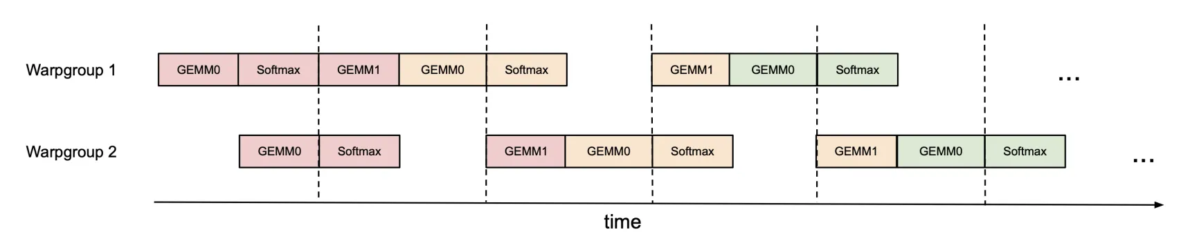
In fact, this already forms ping-pong scheduling: the producer warp is responsible for loading the next K/V tile (and occasionally the next Q tile) via TMA into the buffer region of shared memory (there are two buffers in total, which we call the A/B buffers), while the consumer warp is responsible for performing the GEMM asynchronously with wgmma.mma_async, followed immediately by the softmax operation (note that the algorithm has already simplified this operation to maintaining the two variables m and ℓ; of course, what’s ultimately stored is the single variable L).
If we picture an asynchronous task pipeline model, we’ll see: the producer writes A; the consumer computes A while the producer writes B; the consumer computes B while the producer writes A… and so on, round and round. This is pingpong-scheduling. The waits for their asynchronous operations are implemented with mbarrier, i.e., instructions like bar.sync.
The next question to address is: it’s easy to understand that TMA and data movement can be asynchronous with computation, but why can GEMM also be asynchronous with softmax? If we think about it from the hardware perspective, we can answer this:
wgmma.mma_async uses the Tensor Cores for computation
Although Softmax has been simplified by the algorithm into this form where only a few variables need to be maintained, it’s still a general-purpose computation, which runs on the Cuda Cores (strictly speaking, the compute units include: Cuda Cores, FP ALUs, SFU)
Tensor Core and Cuda Core computations can overlap; they don’t contend for resources, so there’s no problem
Hence, we get the following timing model:
5.2 intra-warpgroup overlap
In fact, after analyzing the algorithm’s dependencies, we can go a step further with overlap optimization. The paper directly breaks these dependencies to achieve further asynchronous overlap; let’s see how it’s done:
First, in the initial stage, compute Scur=QiK0T and P~cur,ℓi, and rescale Oi
for loop: (note: the steps that wait on asynchronous loading are omitted here; we focus on the computation logic)
Compute Snext=QiKjT — this computes the S of the next block; issue it without waiting
Compute Oi=Oi+P~curVj−1 — this computes the current O, since P~cur was already computed in the previous stage (either the previous loop iteration or the initial stage outside the loop)
Based on Snext, compute mi,P~next,ℓi — this step is the softmax computation
Compute P~curVj−1 and wait, then rescale Oi
Release the buffer
Copy Snext into Scur‘s position, ready for the next loop iteration’s computation
end loop
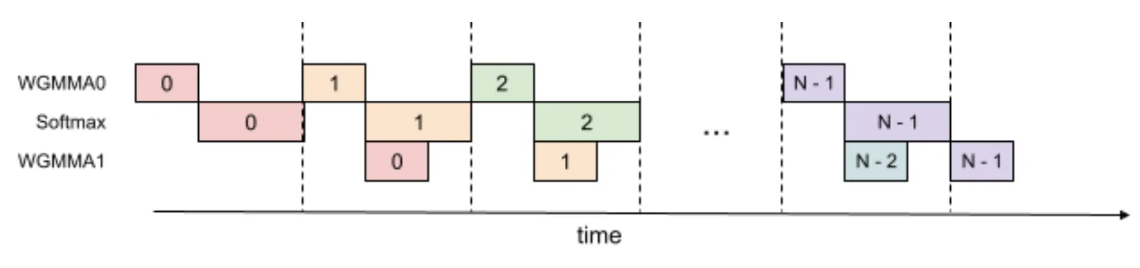
So in effect, within one loop iteration the Tensor Cores are computing two blocks’ worth of work: the current block’s P~curVj−1 and the next block’s Snext=QiKjT. If we visualize this timing task graph on the pipeline, it looks like this:
On the H100, wgmma.mma_async (Tensor Cores) and the exp/scaling in softmax belong to different functional units, and their throughput/latency is actually very asymmetric: for example, in a typical configuration, MUFU.EX2 (exp2) takes about 1500 cycles, while one WGMMA costs more than that, at 3072 cycles. If the softmax part is tucked into WGMMA’s “shadow”, the whole pipeline stays fuller.11
Earlier, through ping-pong scheduling, we raised throughput from 580 TFLOPS to 640 TFLOPS; then, with this intra-warpgroup reordering, throughput goes up to 670 TFLOPS.
5.3 Using FP8
The main reason to use FP8 is really that it computes faster, but two problems and challenges immediately arise:
How do we arrange the data into the layout required by FP8 wgmma, to saturate the tensor cores?
FP8 computation loses a lot of precision; how do we keep that loss as low as possible?
layout conformance
At the PTX level, wgmma imposes mandatory constraints: the accumulator is specified as FP32, and FP8 has a minimum tile size. In practice, the Q,K,V we compute with are usually contiguous along the head dimension, so feeding them directly into wgmma.xxx.mXnXkX leads to misalignment and discounted throughput. The paper’s solution is to transform the layout so that the data lines up:
For V, it must be contiguous along the sequence dimension seq_len in shared memory. Since TMA can’t do transpose + load, FA-v3 performs the transpose inside the kernel, converting the V tile from head-major to seq-major; this step is done in the producer warp.
FA-v3 does a byte-permute inside registers or shared memory to reorder the accumulator, so that it matches the data format required when it is fed in as input the second time.
Accuracy
To curb the precision loss, FA-v3 proposes two schemes:
block quantization: compute the scale factors for Q,K,V separately on a per-block basis and perform FP8 quantization within each block. Compared with per-tensor scaling, this scheme adapts better to dynamic local ranges, introduces no extra write operations, and can be fused with operations such as RoPE.
Incoherent Processing: before quantizing to FP8, multiply the same side of Q,K by a random orthogonal matrix M, and multiply by MT after quantization. Since M is orthogonal, this doesn’t change the final result of the attention computation, but it spreads the outliers out across coordinates.
With FP8, throughput is pushed to 1.2 PFLOPS, and the error is 2.6× lower than the baseline.
On FP8 Attention, I recommend checking out the Sage Attention series of papers; this is also what I reproduced and enhanced during my time at Paddle, and overall it’s a pretty solid piece of engineering work.
Appendix: Interview Rapid-Fire Q&A
No need to write a conclusion — if you’ve read this far, you already have a good grasp of the optimizations in the FA series. Let’s do something useful instead: if an interviewer grills you on Flash Attention again, can you answer the following questions?
What is FA-v1’s partitioning scheme for KV?
A: Split KV column-wise and Q row-wise, while reusing KV on-chip.
What optimization did FA-v1 propose for softmax to reduce the cost of maintaining variables?
For each query row, only three variables need to be maintained: m,l,r
Within a segment: mt=max(x(t)),ℓt=∑ex(t)−mt,rt=∑ex(t)−mtV(t)
This way, there’s no need to keep the intermediate results S,P, both of which are N2-sized data; this reduces the number of IOs and also lowers GPU memory usage.
What optimizations did FA-v2 make?
Adding seqlen as a parallel dimension: slice the computation more finely so that more independent tile instances can run concurrently, improving SM occupancy and pipeline efficiency (especially with a small head dim and long sequences).
A better parallelization strategy: optimize on-chip data reuse, going from warps accessing KV to warps accessing Q and sharing KV, which reduces shared memory round trips and synchronization.
Skipping based on the causal mask: skip whole blocks in the upper triangle, and apply element-wise masking only on the diagonal blocks; most blocks are either “fully computed / fully skipped”, so there’s less branching.
A more I/O-efficient backward pass: apply recomputation systematically; the bwd pass doesn’t store P or S either, but recomputes the QKT segments on demand and accumulates dQ,dK,dV online.
Talk about FA-v3’s warp-spec
Producer: use TMA to asynchronously move the next K/V block (sometimes also a Q slice) into shared memory, with two shared memory regions set up as buffers;
Consumer: run WGMMA (QKT) on the other buffer, squeeze softmax into the gaps, then run WGMMA again (softmax × V).
Are you familiar with FA-v3’s intra-warpgroup overlapping? Talk about it — in particular, what does it do compared with the original warp-spec? What insights did you take from it?
After analyzing the concurrency bottleneck, it breaks the earlier algorithmic dependencies, computing the current PV and the next block’s QK at the same time while overlapping them with softmax, and uses wgmma’s asynchrony + TMA’s asynchrony + the SFU for softmax to further break down the granularity of pipeline parallelism.
Difference: 3.1 addresses cross-group Producer/Consumer concurrency; 3.2 then squeezes out the air gaps within a group, eating up the tiny holes between WGMMA and softmax.
Insight: when you hit a program bottleneck, especially an asynchrony bottleneck, analyze the sequential dependencies, flexibly emulate FA-v3’s asynchronous techniques, and interleave the different Tensor Core and Cuda Core compute tasks for finer-grained optimization.
How does FA-v3 do its FP8 optimization? How does it reduce the precision loss?
On the layout side: transpose the V tile in the producer warp, and at the same time reorder the accumulator registers to fit the FP8 input, so that both GEMMs can meet the requirements of wgmma’s FP8 instructions.
On the loss-reduction side: do block scaling, and also multiply by an orthogonal matrix + its transpose. Although this introduces extra computation, it spreads out the precision loss, which makes it a worthwhile trade-off.