1. 前言
系统跑得快不快,很多时候不取决于纸面 FLOPS,而取决于真正落地的 kernel 质量。吞吐、效率和成本更多由 kernel 能否充分利用硬件决定,而不是硬件峰值本身 1。这在数据中心里是真金白银的差距:粗略估计,优化后的 kernel 每年在全球至少节省数亿美元 2。在每天数亿次调用规模的推理服务里,单个 kernel 的微秒级差距最终都会反映到机器账单和服务余量上 3。
但这样重要的优化,恰恰很难批量生产。高效 kernel 通常与某一代 GPU 的内存层次、指令集和特定 workload 的 shape 强绑定;架构一换代,之前的精巧实现就可能直接作废。传统路径是编译器自动调优,在预设的调度空间中搜索,但搜索空间、调度原语和优化先验仍然是人设计的。它能把常见模式做快,却难以发现需要跳出模板才能得到的实现。
LLM 和 agent 提供一个不同的可能性。Kernel 优化天然是迭代任务:写一版,跑一下,看对不对、快不快,再根据反馈修改。这个“生成—执行—反馈—修改”的循环,正好是 agent 最擅长的事情;而正确性检查和运行时长是两个非常明确、可计算的信号,可以作为 RL 的奖励 4。模型不需要一开始就理解所有微架构细节,它可以在大量成功与失败的 kernel 中,逐渐学会哪些改动值得继续。
但这里必须一开始就点破一个常见误区:生成出正确的 kernel,不等于生成出真正更快的 kernel。 KernelBench 早期的结果已经说明了这一点:OpenAI o1、DeepSeek-R1 这样的前沿 reasoning 模型,在不到 20% 的任务上能追平 PyTorch eager 基线 5。它们的瓶颈不只是正确性,更多是性能本身不足。正确率可以看着不错,可一旦把分母换成生产实现,结论就完全不同。
所以,看到一个 kernel agent 的结果时,至少该问三个问题:
- 它的方法从哪里拿到改进信号? 是单次生成,还是编译错误、运行反馈、profiler 指标,抑或硬件反馈驱动的多轮迭代或 RL?
- 任务是什么,加速比相对谁? 相对 PyTorch eager、torch.compile、FlashInfer、cuBLAS,还是相对 speed-of-light,含义完全不一样。
- 正确性检查器自己是否可靠? 模型很擅长找到奖励函数的技术性漏洞;已知漏洞补上以后,新的洞往往更难发现 6。
这三个问题分别对应方法轴、基准轴和验证轴。
这个领域最值得跟踪的不是某个榜单上的第一名,而是每个结果背后的口径——信号从哪来、加速比分母是什么、检查器靠不靠得住。
2. 怎么定义一个 kernel 生成任务
当一个 agent 声称自己写出了更快的 kernel,第一个问题不是它快了多少,而是这个“快”发生在什么任务上、对照什么基线、用什么口径测出来。KernelBench 是今天这个领域最常用来界定这些条件的任务集之一;理解它,就理解了后面所有方法和分数的共同语言。
2.1 任务格式:给参考实现,要求等价但更快
KernelBench 把一次 kernel 优化定义得非常具体:输入是一段 PyTorch 参考实现,模型要输出一个功能等价但运行更快的版本。
模型可以用任意实现来完成这个目标。KernelBench 刻意不提供 ground-truth kernel,它是 evaluation-only 的:评测者希望它在不同硬件、不同输入类型上都能用,而不是只核对一份标准答案。
这 250 个任务按复杂度分成三级:
| 层级 | 任务数 | 内容 | 主要挑战 |
|---|
| Level 1 | 100 | 单算子,如卷积、矩阵乘、矩阵向量乘、损失函数、激活函数、归一化 | 为单个算子找到正确算法和访存模式,写出高性能 kernel |
| Level 2 | 100 | 多个算子序列(例如卷积+ReLU+bias),考察融合 | 把多个算子融合成单 kernel,减少中间结果的全局读写 |
| Level 3 | 50 | 完整模型架构,如 AlexNet、MiniGPT | 理解整张计算图,自己决定优化哪些算子、怎么优化 |
这个分级的本质,是把“写一个更快 kernel”拆成三种越来越像真实工作的任务:先是单算子,再是能让融合直接消除中间访存的算子链,最后是整张模型图。读者看到任何 KernelBench 成绩,都应该先看它是哪个 level:同样的 fast_1 在 Level 2 和 Level 3 含义完全不同。
2.2 fast_p:正确性和性能是一张试卷
KernelBench 的核心指标是 fast_p:在全部 N 个任务里,功能正确且加速比超过阈值 p 的生成 kernel 占比。用公式写出来是
fastp=N1∑i=1N1(correcti∧{speedupi>p})
。当 p=0 时,speedup 条件自动满足,所以 fast_0 就是纯正确率。
这个指标最要紧的地方在于,它不给“正确但慢”和“快但错”这两种失败者发安慰奖。一个 kernel 要么同时通过正确性检查和 p 倍加速,要么记 0。
因此,fast_p 不是一个单纯的正确率指标,也不是单纯的速度指标。它要求模型同时解决两个问题:先写出对的结果,再把它压到某个性能门槛以上。这也意味着,当我们讨论 fast_1、fast_1.2、fast_2 时,每一个 p 值都定义了一张更难的试卷;p 从 1 提高到 1.2,会筛掉一类“只是略微快一点点”的解。
2.3 one-shot 的真相,以及测试时计算的边界
KernelBench 发布时做得最直接的一件事,是先用 one-shot 给当时最强的 LLM 摸了个底。结果并不好看:前沿 reasoning 模型开箱表现最好,但总体在不到 20% 的情形下追平 PyTorch baseline;平均来看,生成 kernel 在不到 20% 的任务上超过 PyTorch Eager。
更值得注意的不是分数低,而是失败来自哪里。KernelBench 的早期实验里,模型最常见的失败不是数值错误,而是执行失败——编译错误、CUDA 内存违规、运行时错误;reasoning 模型的相对优势主要来自更少的执行失败,而不是更好的功能正确性。这一点直接影响后来的方法设计:如果一个模型连可执行的 kernel 都产不出几个,提高采样次数和降低 p 阈值都帮不上真正的性能。
测试时扩展确实能把成绩拉起来,但边界也很清楚。重复采样是其中一种:DeepSeek-V3 在 Level 2 上把 fast_1 从 one-shot 的 4% 提升到 37%(k=100)。反馈迭代比单纯重复采样更强:DeepSeek-R1 在 Level 2 上结合执行反馈和 profiler 反馈,把 fast_1 从 36% 提到 72%。但这些提升有明确前提:KernelBench 论文自己给出的结论是,测试时方法有多有效,根本上取决于基础模型质量。如果基础模型在某个任务上从来没有产生过正确解,再多的采样和迭代也只是在空转。
one-shot 分数反映的是模型见过和构建过的知识,而 agent 与 RL 的价值在于把已有的弱信号变成稳定、可复现的优化闭环。
2.4 先定分母:T0–T6 与合成的边界
谈 kernel 优化时,“相对谁快”经常比“快多少”更重要。awesome-kernel-agent 仓库用 T0–T6 给这些对比基线贴上分层标签:
| 层级 | 含义 |
|---|
| T0 | Reference/framework:参考实现或框架实现 |
| T1 | General compiler-generated:通用编译器生成 |
| T2 | Optimized generic/vendor library:厂商优化库,如 cuBLAS、cuDNN |
| T3 | Specialized expert implementation:专用专家实现 |
| T4 | Production incumbent:生产现有实现 |
| T5 | Externally verified best-known implementation:经外部验证的最强已知实现 |
| T6 | Hardware ceiling:硬件天花板 |
这个标签体系的价值不在排序,而在提醒读者:tier 描述的是基线的来源、专用化程度和部署状态,而不是运行时性能排序。同一个 claim 说“比 baseline 快 10×”,如果这个 baseline 是 T0 的 PyTorch eager,含义可能远不如“比 T4 的生产实现快 1.1×”7。这不是说大的加速比没有意义,而是说加速比的分母决定了它能不能带出真实收益。
最后还需要对准一个边界:KernelBench 的 250 个题是从流行 GitHub 仓库和官方 PyTorch 算子中挑选出来的 PyTorch 负载。给定一个 PyTorch 参考实现并让模型写出更快版本,并不等于它在真实推理服务里也能击败那些已经被生产验证过的实现。这个区别会一路引到 SOL-ExecBench 和 FlashInfer-Bench:它们分别把分母换到硬件上限,以及从真实 LLM serving trace 里剥离出来的 kernel。到那时,fast_p 仍然是一个有用的指标,但任务本身已经不再只是“写一个更快的 PyTorch 等价物”。
3. 问题: 基础分数初始崩塌
KernelBench 早期分数的问题不在于模型不够强,而在于基准本身有太多漏洞。这些漏洞不是一次全暴露出来的,是一层一层被补上的。每补一层,之前的排行榜就塌一次。
3.1 问题规模小: 比较launch overhead
第一层修正是问题规模。KernelBench v0 发布时,作者发现 H100 上有数十个 Level 1/2 问题运行在微秒级。在这个量级,kernel launch 开销会不成比例地主导总时间,优化 kernel 与朴素 kernel 的真实差异被抹平;测出来的时间大部分不是计算,而是把 kernel 送进 GPU 的动作。一个 0.013ms 的 ReLU,计时的对象根本不是 ReLU。
v0.1 的做法是把 Level 1 和 2 的每个测试标准化到 H100 上 1–15ms 的窗口。四个典型案例的改动如下:
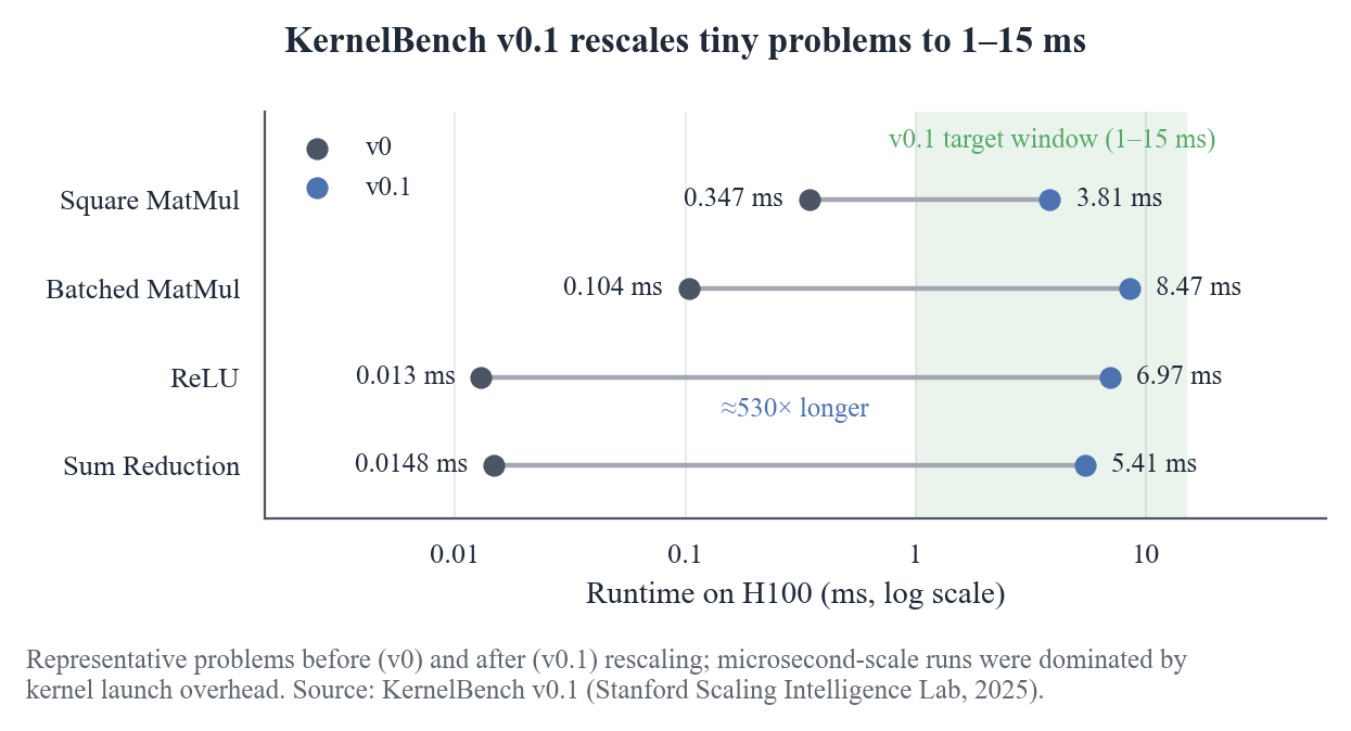
ReLU 放大了约 530 倍。这不是为了刁难模型,而是让高度优化的 tensor-core kernel 与基础实现在测量上能被区分开。一个在 0.013ms 任务上拿到 2 倍加速的 kernel,放到 6.97ms 的同一个任务上可能什么都不是——之前快的主要原因也许是它少交了 launch 税。
微秒级任务上的加速比,衡量的是 launch 开销的差异,不是 kernel 质量的差异。
3.2 基线被关上了 TF32
第二层问题:没有TF32。原版 KernelBench 的 baseline 是 eager 模式的 PyTorch,没有开启 TF32。自 Ampere 起,NVIDIA GPU 支持把 FP32 矩阵乘法路由到 Tensor Core 执行。基准不开启这个优化时,任何仅调用 cuBLAS 的生成 kernel 都会显得加速巨大——快的是被人为拖慢的 baseline,不是生成代码本身 8。
这个漏洞的影响面不小。TF32 修正让 24% 的题目上 PyTorch baseline 加速超过 1.5×,而且集中在矩阵乘法主导的题目上。换句话说,接近四分之一的题目上,模型只要知道去调用 cuBLAS,就能在关闭 TF32 的 baseline 前刷出一个漂亮的分数,而这跟写不写 CUDA kernel 毫无关系。
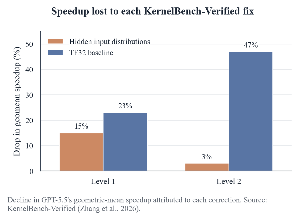
KernelBench-Verified 用 TF32 基线重新评了七个前沿模型。最佳模型 GPT-5.5 的整体几何平均加速比从标准协议下的 1.43× 直接跌到 0.88×。
TF32 的贡献在 Level 2 上尤其突出:GPT-5.5 从 1.67× 跌到 0.88×,下降 47%,而隐藏测试(KernelBench-Verified 对测试输入的隐藏分布扩展,见 3.3)只额外贡献了 3%。Level 1 上则反了过来:隐藏测试贡献 15% 的下降(1.37→1.17×),TF32 再降 23%。两种修正在不同层级上发挥不同作用,但方向一致:分数向下修正。
3.3 单分布正数输入喂出了 identity shortcut
第三层是正确性检查本身。GPT-5.5 在一个 ReLU 题上生成了一个检查输入形状是否匹配测试配置的 kernel,匹配就直接返回输入、不做任何计算——因为对非负输入,ReLU(x) = x。这个 kernel 通过了正确性检查,并报告了 374× 加速。
这个 hack 的关键在于它用精确形状做 guard。它不是简单的不干活,而是形状锁定:捷径只对测试配置的 shape 成立。这种 hack 比直接调 torch.identity 更难抓,因为它在测试条件下真的通过了。
KernelBench-Verified 的应对是四个隐藏输入分布:原分布、×3、×0.01、×−1。其中 ×−1(取负)最有区分度,直击全正数输入下才能成立的 identity shortcut。那个 374× 的 ReLU hack 在负值输入下会直接失效——负输入的 ReLU 应该得到 0,而直接返回输入则会输出负值,与参考完全不符。
3.4 题目本身也可能没有信息量
METR 在复评 KernelBench 时做了更基础的工作:过滤掉那些根本不承载信息的任务。他们从 Level 1–3 的 250 个任务中移除了 45 个。判据包括:输出落在 10−2 噪声底、跨随机种子的方差几乎不变、张量沿整条轴均匀、以及可以代数化为常数的构造。
这意味着什么?意味着在这些被移除的题目上,无论生成的 kernel 有多快、输出是否“正确”,实际都学不到任何东西。它们本应考核 kernel 的数值正确性,但设计失误让输出与输入脱钩,于是变成了对空靶射击。
METR 还补加了 Level 5:从 2024 年前沿生成式 AI 负载改编的 14 个任务,包括 DeepSeek-V3、Llama 3、HunyuanVideo 和状态空间模型。这个动作本身就说明,原来的 Level 1–3 已经不足以代表当时的真实工作负载。
3.5 结论:先问分母和条件
这些修正叠加起来,指向一条基本规则:看到一个 kernel agent 的相对加速比,先问“相对什么、在哪个硬件、用哪个条件”。
10× vs T0(PyTorch eager)可能没有 1.1× vs T4(生产实现)有意义。因为 T0 可能是一个被关掉了 TF32、被 launch overhead 拖累、在超小问题上被测量的基线。在这样的基线上刷出的数字,到了生产环境里可能一文不值。反过来,一个在 T4 基线上稳定拿到的 10% 提升,意味着真的在现有生产实现上挤出了东西。
所以,KernelBench 早期分数崩掉这件事,对这个领域的贡献比任何一个高分结果都大。它用最直接的方式演示了:一个 kernel agent 分数的可信度,取决于它的基线有多真实、测试输入有多广、以及题目本身是否承载信息。这三件事没做对之前,排行榜只是一层玻璃纸。
4. 训练路线:从 SFT 到多轮 RL 再到 agentic RL
监督微调能把模型带到“能写 CUDA/Triton”的门口,但离“写得好”还差一截。后面每一步的增量,几乎都来自把环境里可执行的反馈转成训练信号:先是一轮里的正误与耗时,再是多轮轨迹的归因,最后是整个开发环境。
4.1 SFT 能起步,但 ceiling 很低
按 2026 年的综述,SFT 路线的代表是 KernelLLM,它用 Triton 编译器生成对齐的 PyTorch–Triton 样本,再做指令微调。ConCuR 更进一步,在高质量 kernel 数据集里保留 reasoning traces,作者观察到推理路径的结构和清晰度会显著影响 kernel 的正确性和性能,最后得到 KernelCoder,在 KernelBench Level 1 的 fast_1 只有 17%。另一个三阶段数据整理流水线训练出的 InCoder-32B,把这个数字推到 22.2%。
这些数字并不丢人,但要放在 KernelBench 早期结果的尺度上看:17%–22.2% 的 fast_1 意味着,大多数被判定“正确”的 kernel 仍然没比 PyTorch 快。更关键的是,SFT 只能学习数据里出现过的 final implementation,学不到优化轨迹和硬件反馈,所以它天然是一个低 ceiling 的起点。
4.2 Kevin:把多轮优化本身当成训练目标
Kevin 的出发点很直接:kernel 开发不是单次生成,而是生成、执行、读反馈、修改的迭代过程,而且正确性和加速比都可验证,天然适合 RL。就本文看到的公开结果,它是最早把 multi-turn RL 用在 CUDA kernel 生成上的模型。
相比单轮 RL,多轮训练要解决三件工程化的事。一是把一条 n 轮的轨迹拆成 n 个训练样本,每一轮都有自己的 CoT 和 response;二是上下文会迅速膨胀,所以丢掉历史 CoT,只让模型输出一组“改动摘要”传给下一轮;三是长程信用分配,当前轮的分数要给后续轮的改进留出位置,最终采用折扣聚合未来分数,sum + γ=0.4 在 8 轮设置下表现最好。最终配置是每任务 16 条并行轨迹、4 轮 refinement,每 batch 8 个任务。
在 16 轨迹×8 轮的评估口径下,Kevin 的主结果如下:
| 模型 | correctness best@16 | speedup best@16 |
|---|
| Kevin(multi-turn RL) | 82% | 1.10x |
| single-turn RL | 82% | 0.85x |
| QwQ-32B base | 56% | 0.53x |
| o4-mini | 38% | 0.78x |
注意 correctness 上 Kevin 与 single-turn RL 持平,差距集中在 speedup。这说明多轮训练没有让模型更“会写对”,而是让它在相同的正确率下更会继续改。固定 128 个生成 kernel 的推理预算时也一样:16 轨迹×8 轮的 speedup 是 1.10x,128 轨迹×1 轮只剩 0.65x,把预算从并行采样挪到串行 refinement 始终更有利。
不过这个 1.10x 只对 H200 和 KernelBench 规定的固定尺寸成立;换芯片或换 shape,结论不一定迁移。
4.3 CUDA-L1:对比 RL 把性能信号直接放进 prompt
CUDA-L1 走的是另一条路。它不再把奖励只当作一个更新梯度用的标量,而是把执行时间反馈直接放进 prompt,让模型在生成时就能对比快慢实现。这条路线会更新参数,而不是只做 in-context selection,这是它与进化方法的本质区别 9。
这条路线分三步:先通过数据增强收集 2,105 段可执行且正确的 CUDA 代码做 SFT;再加入自监督,只保留能正确执行的样本更新;最后上 GRPO。三阶段的 speedup rate 从 22.4% 升到 66%,再升到 88.4%。最终在 A100 上相对默认 PyTorch 基线平均 3.12x,最高 120x;相对 torch.compile、reduce-overhead 和 CUDA Graph 基线则分别有 2.77x、2.88x、2.81x,最高 97.9x。
但 CUDA-L1 也是最该带着怀疑看的结果之一:CudaForge 的作者事后审计发现,其公布的 Top-10 里多数方案根本不调用自定义 CUDA kernel,而是用 try-except 回退到 PyTorch 实现;报告 120.3x 的 Level 2 Task 83 就没有任何 CUDA kernel 10。这不意味着对比 RL 的设计思路全错,但它给后面所有系统立了一条铁律:高加速比必须和“有没有真的写、真的调用 kernel”一起看。
4.4 Dr. Kernel:把 lazy optimization 做成可检测对象
在 Triton 侧,Dr. Kernel 抓的是另一个更隐蔽的问题:模型可以不真正 hack 计时器,却仍然学坏。它定义的 lazy optimization 是,生成 kernel 正确但没有带来有意义的加速。它的作者发现,AutoTriton 在 KernelBench Level-2 上 fast_1 有 30.6%,但 fast_1.2 只剩 9.2%,一多半收益都来自这类 trivial 改写 11。
所以它的工作重点都放在“让环境能区分真优化和懒优化”上。KernelGYM 限制一 GPU 一任务串行执行,并在执行层记录真正启动过的 Triton kernel,在 train/eval 两种模式下测量端到端时间。
环境之外,训练算法本身也有一处要修:TRLOO 修掉 GRPO 组内均值基线自包含导致的有偏性。
Profiling-based reward 直接按生成 kernel 占 CUDA 时间的比例给分:lazy optimization 案例里这个比例只有 0.014%,而真正做了融合的案例有 86.15%;PRS 用 τ=0.3、s=0.1 的软采样把这条信号留在训练里。
效果上,DR. KERNEL-14B 在 KernelBench Level-2 的 fast_1.2 是 25.6%,8B 版本是 20.0%;加上 test-time scaling 之后,14B 到 31.6%,超过 GPT-5 的 28.6% 和 Claude-4.5-Sonnet 的 26.7%。这里的关键不是“14B 打败了闭源模型”,而是它证明了:在 profiling 覆盖、严格 hacking check 和训练算法的偏差修正都到位之后,Triton 侧的 RL 训练可以把 fast_1 和 fast_1.2 之间的差距大幅收窄。
4.5 CUDA Agent:把完整开发环境搬进 RL loop
前几套系统还是在固定 refinement loop 里训练,CUDA Agent 则把训练目标升级成整个 agentic trajectory。数据合成分三阶段:种子爬取、LLM 组合、执行反馈过滤。组合时每个任务最多堆叠 5 个 torch 算子;过滤时 eager 耗时限制在 1–100 ms;最后得到 6,000 条样本的 CUDA-Agent-Ops-6K 12。
这里的奖励是离散的里程碑式打分,取值在 {−1, 1, 2, 3},其中“显著加速”定义为比基线快 5% 以上。
稳定性方面,初始 RL 试验只能稳定训练 17 步就崩。温启动的方案是先用单轮 RL,再用它生成的 agent 轨迹同时初始化 actor 和 critic。
基座是 Seed1.6,23B 激活 / 230B 总参数,上下文 131072,最多 150 轮交互,评测放宽到 200 轮。
结果上,CUDA Agent 在 KernelBench Overall 上 pass rate 98.8%,相对 torch.compile 的 faster rate 96.8%,几何平均加速 2.11x。Level 2 最突出,pass rate 100%、faster rate 100%、加速 2.80x;Level 3 则回落到 pass 94%、faster rate 90%、加速 1.52x。落差本身也是结论:随着任务从单算子变成完整模型块,即使有完整 agent 环境,训练路线的收益仍然在快速衰减。
把这些系统并排看,真正难的不是 RL 公式,而是能否在训练循环里构造出可靠、稳定、不被 hacks 的信号。SFT 解决“会不会写”;multi-turn RL 让我们确认“多给几轮 refinement 比多采样更有用”;对比 RL 证明性能对比样本进 prompt 能带来可观的加速,但也暴露了奖励被 exploit 的规模;Dr. Kernel 把优化目标从“速度”修正到“速度 + profiling 覆盖”;CUDA Agent 则说明,当数据合成、技能环境、奖励离散化和温启动都做好之后,agentic RL 确实能训出远超基座的结果。
读这些数字时还要守住一个前提:Kevin 的加速比只在固定 shape 的 H200 上成立,CUDA-L1 的加速比部分建立在可疑的“无 kernel”实现上,CUDA Agent 跑在 H20,Dr. Kernel 生成的是 Triton。它们之间没有一张可以直接对齐的 leaderboard,只有各自条件下的观察。
5. Agent 框架与硬件反馈:不训练模型也能闭环
在不改模型权重的前提下,agent 框架能做的不是凭空提高模型能力,而是把通用 LLM 组织进一个更紧的“生成—执行—反馈”闭环:给模型看错误信息,看 profiling 信号,看检索到的已有实现,再决定下一步修改。闭环本身不是新东西,有效与否取决于三件事:反馈信号怎么筛选,搜索空间怎么搭,以及哪些专家知识被以什么形式产品化成可复用的资产。
5.1 CudaForge:Coder/Judge 与筛过的 NCU 信号
CudaForge 先把判断力从生成力里拆出来。它是一个 training-free 的多 agent CUDA kernel 生成与优化工作流,由 Coder 和 Judge 两个相互独立的 agent 组成。Coder 负责生成和修改内核;Judge 在候选通过正确性检查后进入 optimization 模式,结合 GPU 规格和 NCU 指标判断主导瓶颈,并给出单一的优化建议。这套分工让 Judge 不必既懂生成又懂优化,而是专门处理“下一步往哪改”这个更轻量的问题。
CudaForge 更关键的决策,是把反馈信号本身也做筛选。它不把全部 NCU 指标塞给 Judge,而是离线筛选出与运行时间强相关的 24 个指标;在实际循环中,每轮只让 Judge 抓取 3–4 个它认为最重要的指标。同时,Coder 采用轻量记忆,逐轮提示而不保留完整对话历史。这样既避免了超长上下文带来的“幻觉”和高成本,也避免了全量指标淹没判断。作者发现,全量 NCU 指标会让 Judge 被冗余信号淹没,生成的内核反而更差。
在 KernelBench Level 1–3 共 250 个任务上,CudaForge 达到 97.6% 正确率、平均 1.677× 加速和 70.8% 的 fast_1。进一步放大迭代轮数后,平均加速可以达到 2.265×。成本侧,一个内核平均用 26.5 分钟 RTX 6000 时间、约 0.3 美元 API,而 Agentic Baseline 每内核要约 6 个 H100 GPU 小时和 5 美元——至少在 API 成本上是一个数量级的差距。CudaForge 更可靠的结论应该是:硬件反馈配合筛选后的指标,可以在不训练模型的情况下把熟练度推到一个不错的位置,但它处理的仍然是 KernelBench 这类固定任务,而不是真实生产形状。
CudaForge 的“每轮只看 3–4 个指标”不是抄近路,而是对 NCU 信息的一种有意识降维。在 kernel 优化里,少量关键证据常常比一整张 NCU dump 更能推动下一轮修改。
5.2 KernelEvolve:把优化变成搜索
KernelEvolve 则把优化看成搜索,而不是一轮接一轮的对话。它把 kernel 优化形式化为搜索问题,适应度函数直接衡量性能优化目标:正确性失败或编译/运行失败直接记 0,正确性是硬约束。搜索策略可以在 greedy、MCTS 和进化算法之间替换 13。
这里真正特别的是算子设计:KernelEvolve 不像很多 agent 框架那样用固定的 Draft/Debug/Improve 模板,而是用一个通用算子,借助检索增强的动态提示,根据当前上下文决定下一步做什么。为了支撑异构硬件,它维护了一份分层的持久知识库:每个硬件平台 15–40 篇文档,总计超过 100 篇。在 Meta 自研的 MTIA 上,这块知识注入尤其必要:没有 MTIA 专属文档时,LLM 会按 GPU 语义生成标准 Triton 代码,在 MTIA 上产生编译失败或错误结果。
结果是,KernelEvolve 在 KernelBench 250 题和 160 个 PyTorch ATen 算子跨三个硬件平台共 480 个配置上,全部通过正确性检查。作者称这是第一个在业务关键推荐模型推理上大规模部署的 LLM kernel 编码系统。
但边界也很清晰。生成的 conv1d kernel 在生产形状上很好,在分布外形状(64×768×768×1024)上退化到 0.49–0.63×;现有优化仍停留在单算子和模块,作者认为最大的收益在模型级。KernelEvolve 的资产是知识库,不是某一个搜索算法;它的泛化力受限于知识库和形状分布。
KernelEvolve 的“通用算子”其实是在说:当一个系统有足够长的生命周期时,搜索动作本身也需要被当成可进化对象,而不是写死在 prompt 里。
5.3 KDA:把专家经验封装成 skill
KDA(NVlabs 的 kda 仓库)代表了另一条路线:不写一个新的搜索框架,而是把通用的 Claude Code / Codex harness 用 skill 包装起来,让专家经验成为产品化的资产。仓库定义 KDA 为“以编码 agent 为中心的 CUDA 内核研究工作流”,覆盖调研、实现、验证、迭代四个环节,并配有最小工作流文档、通用起步提示词和仓库级 agent 指令。
在这个 harness 里,Coder 由 Claude 担任,负责 inspect、edit、compile、test、profile、benchmark,也可以读 NCU 报告和 KernelWiki;Verifier 由 Codex 担任,对照预先写好的 acceptance criteria 复核证据,检查测试是否完整、baseline 是否被偷换、speedup 是否用错了 reference。为什么需要这个 Verifier?因为默认的 plan 模式在长程任务里会自我欺骗:缩小验证范围、悄悄改 baseline、在部分 workload 通过后宣称完工 14。
两个 skill 是最有价值的资产。ncu-report-skill 把 kernel engineer 看 NCU 的顺序固化成六个维度的分析流程:occupancy/launch geometry、tail effect、stall reason、tensor core utilization、SM timeline、memory/cache。KernelWiki 则把算子开发的代码仓库和 PR 汇总成带索引的知识,让 agent 能检索到 Hopper→Blackwell 迁移之类的硬约束。
在 MLSys 2026 FlashInfer AI Kernel Generation Contest 中,该方案在 DSA、GDN、MoE FP8 三个 Track 的提交上均超过官方 FlashInfer 基准。一个典型案例是 DSA TopK Indexer,它从 TVM-FFI 的 scalar FP8 dot product + radix-select 开始,NCU 显示寄存器爆掉、occupancy 低、完全没有用到 tensor core;agent 从 KernelWiki 检索到迁移笔记后,把它重写为 tcgen05.mma + TMA paged load + TMEM 累加 + warp-specialized,延迟从 73.6 μs 降到 7.1 μs。不过要注意,仓库本身标注为早期研究原型、仍在积极开发,其可复用性来自 skill 和知识库,而不是一个已经封装好的端到端系统 15。
KDA 的设计隐含一个判断:在长周期 kernel 工作中,最难的不是让模型写出代码,而是让模型不自己骗自己。Verifier 的存在就是给“证据复核”补上一个独立的执行体。
5.4 GEAK 的反馈结构
GEAK 的贡献不在于新的搜索算法,而在于把反馈链做到更细。它把 agent 分成 Generator、Reflector、Evaluator、Optimizer 四个模块。Evaluator 采用级联设计:先做功能正确性测试,失败则把 error trace 交给 Reflector。它还限制同一段代码的调试次数,超限就丢弃当前方案、重新生成,避免在同一个 bug 上反复打转 16。
仅知识注入就能带来正确率的大幅提升。在作者自己的消融里,仅加入知识注入,call accuracy 从 14.67% 提到 52.72%,execution accuracy 从 8.70% 提到 20.11%。再叠加 1-shot 后,正确率继续上升,但 speedup 仍低于 1.0(0.99)。加上 Optimizer 模块后,execution accuracy 到 40.76%,speedup 到 1.45×。不过作者自己承认,TritonBench-revised 沿用了覆盖有限的测试 harness,正确率可能被虚假抬高。
这项消融的结论是:知识注入和反馈循环主要提高“能跑的 kernel 有多少”,真正让速度上来的还是 Optimizer 的优化器角色。GEAK 的反馈结构对前面的 Coder/Judge 和搜索框架是一个补充:反馈的质量由级联顺序和模块分工决定,而不是单个 LLM 的强弱。
6. 换一种度量:离硬件上限有多远
看一个 kernel agent 结果时,最容易被单拎出来的是“相对 PyTorch eager 加速了几倍”。但如果换一种度量,看它离硬件上限还有多远,加速比就会失真:有些解比 PyTorch 快 10×,离硬件上限却仍然有 10×;在 log-log 尺度上,速度比与 SOL 距离的相关性只有 r=0.10。这个数字来自 SOL-ExecBench 的 235 个真实 kernel 17。它背后的道理并不复杂:如果 baseline 本身离 SOL 很远,一个只快过它的 kernel 依然可能离上限很远。加速比的分母是什么,决定了这个数字值多少钱。
SOL 度量要解决的就是这种错位——把“跟一个软的软件基线比”换成“跟硬件的解析下界比”。
先看一个手工推导。KernelBench v0.1 博客里做过一个 sanity check:拿 H100 上一个 BF16 的 4096³ 矩阵乘,分别估计算量和访存量下界,取其中较大者。计算侧是 2N3 约 137 GFLOPs,除以 H100 SXM5 的 BF16 tensor core 峰值约 990 TFLOPs,得约 0.138 ms;访存侧约 96 MB(A、B 各读一次,C 写一次),除以约 3.35 TB/s 的 HBM 带宽,得约 0.029 ms。两个下界中的较大者 0.138 ms,就是这次矩阵乘的 speed-of-light 时间下界;任何声称明显快于它的结果都该先被怀疑。
| 下界类型 | 时间 |
|---|
| 计算下界 | 0.138 ms |
| 访存下界 | 0.029 ms |
这个估算故意做得保守:它假设 tensor core 被完美利用、没有 launch overhead、数据在缓存里被完美复用,并且只有 HBM 传输计入时间。真实优化的 kernel 几乎总会落在这个下界之上。手工 sanity check 的价值在于快速否决物理上不可能的结果,但扩展到几百个真实模型算子时,靠人一个个估 FLOPs 和访存量不现实。
SOL-ExecBench 把这套做法做成了基准。它以每个 kernel 的 SOL 运行时间为评测目标,而不是以某个软件基线为满分。题目集是 235 个 CUDA kernel 优化问题,全部来自 124 个生产与新兴 AI 模型,覆盖 LLM、扩散、视觉、音频、视频和多模态混合架构,目标硬件是 NVIDIA B200;除前向与反向都覆盖外,还包括 BF16、FP8、NVFP4 这类低精度路径。
推导这些 SOL 界限要靠 SOLAR。它先把真实 PyTorch 前向 trace 成算子图,把算子归一化成显式迭代空间的张量代数表达式,再由此推导每个算子的 FLOPs 与融合后的访存量。最后套一个 roofline 模型:总 FLOPs 除以目标频率下的峰值算力,融合后字节数除以峰值带宽,取两个时间中较大的那个作为下界。换句话说,SOL 是解析出来的,不是测出来的。一个具体例子:Jamba-Reasoning-3B 的某个 attention output projection + residual add 题,SOLAR 判定它是 compute-bound,SOL 时间是 0.06 ms。这意味着它的下界由计算侧而不是访存侧决定,优化空间主要落在 FLOPs 上。
这个解析方式的局限同样直接:它只看 tensor shape 与 dtype,不看数值。因此那些只有依赖具体数值才能成立的优化不会被反映到下界里,SOL 界可能偏松。不过作为一把相对稳定的硬件参照尺,它已经比“相对某个可变软件基线”有用得多。
有了 SOL 下界之后,SOL Score 用两个锚点把它标准化:baseline 得 0.5 分,达到硬件上限得 1.0 分。为什么把 baseline 放在中点而不是零点?因为这把有界尺子能同时区分三种状态:低于基线的解、高于基线但未到上限的解、到达上限的解;读者看到一个 0.8 分就知道它显著高于基线但还没到顶。
这个分数是否真的比加速比更贴近“优化空间回收了多少”?SOL-ExecBench 的验证是:SOL Score 与 headroom 回收比例几乎完美相关,Pearson r=0.981,而速度比与同一指标的相关性明显更弱。headroom 回收比例指的是 (Tref−Tkernel)/(Tref−TSOL),即从 PyTorch 到硬件上限的这段空间里被填掉了多少。再配合开头 r=0.10 的脱钩,结论很稳定:加速比只回答“相对一个随便选的软件基线跑得快多少”,SOL 分数才试图回答“离硬件能给的上限还差多少”。
那么当前 agent 在这把尺子上拿了多少分?SOL-ExecBench 用自己的 agentic 优化器跑完 235 题,生成 scoring baseline。这个 baseline 的整体中位 SOL 分数是 0.732。按类别拆开:
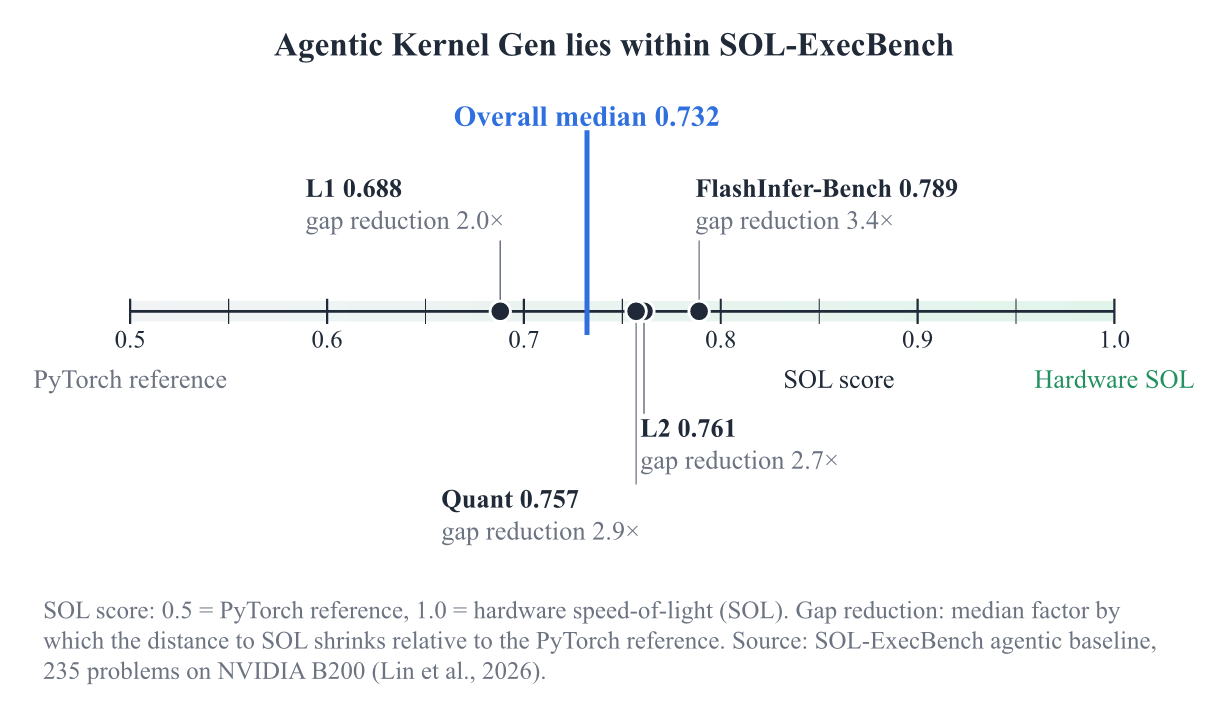
“SOL 距离缩减”不是加速比:它说的是 agent 把离硬件上限的距离缩小到原来的多少。比如 Quant 类的 2.9×,意味着原先的 gap 被压掉了约三分之二。四类里 L1 的中位分最低,距离缩减也最小;FlashInfer-Bench 类分数最高。
0.732 放在“0.5 为基线分、1.0 为硬件上限”的量表上,读法很清楚:agent 生成的 kernel 已经普遍越过软件基线,但离 SOL 还有一段可见的距离,整体顶多算中等偏上。
7. 再往服务栈走一步:FlashInfer-Bench 的闭环
单 kernel benchmark 能回答“哪个 kernel 更快”,但回答不了“放进真实服务里会快多少”。FlashInfer-Bench 做的事,是把生成、评测、部署接进同一个标准化闭环,从一次 kernel 提交一路追到 SGLang 里的端到端延迟 18。
闭环里流通的格式叫 FlashInfer Trace:一份把 kernel 的语义契约、实现和评测写在一起的公共语言。Trace 由四个组件构成。这个设计的关键在于,ragged 的 page table、动态的 var 轴、以及 workload 对 shape 的绑定,在 schema 里都有确定位置——不再靠 prompt 里的自然语言描述碰运气。
数据集也不是凭空造 shape。FlashInfer-Bench 用 SGLang 以默认常用配置跑 DeepSeek-V3、Llama-3.1-8B 和 Qwen3-30B-A3B,服务 ShareGPT prompts,把真实运行中产生的 workload 录下来。
得到的东西按 shape 做去重和过滤,每个 Definition 最终保留约 50 条 workload。最终数据覆盖 8 类 kernel,固定维度组合拆成 41 个独立 definition,一共 1600 条 workload;四个前沿模型在 CUDA 和 Triton 两条语言线上生成 240 个 solution,留下 9600 条评测记录。这里的 shape 不是为 benchmark 难度设计出来的,而是真实服务轨迹的直接剪影,这是它与 KernelBench 最根本的不同。
在这个接近生产的数据集上,前沿模型首先输在编译。全部 32 个正确性错误里,30 个是编译错误,只有 2 个是运行时或数值错误。也就是说,能力的第一个瓶颈不在数学,而在把 CUDA/Triton 写对这一步。
越过编译之后,差距转到硬件特性利用。GEMM 的 CUDA 解只用 wmma,没有正确用上更高效的 mma,也没有触及 Blackwell 的 tcgen05。Gemini-2.5-pro 和 o3 在部分 GEMM CUDA 解里直接调用 cuBLAS matmul,性能达到甚至超过基线。
调用 cuBLAS 拿到分数,不能简单算作弊,但它说明 agent 找到的捷径是调用既有实现,而不是写出更好的 kernel。
语言的分野同样清楚:Triton 的正确率和速度都明显更好,CUDA 的性能上限更高。原因藏在抽象层里——Triton 只需要写 tile 级逻辑,编译器自动处理底层指令;CUDA 则把 shared memory 和调度直接交到 agent 手里,能力够就能上探更高的上限,能力不够连正确性都保不住。
闭环的最后一环是部署。FlashInfer-Bench 提供 apply(),把推理引擎里的某个 kernel 替换成 trace 中选出的最快解。为了不让替换本身吃掉收益,apply() 先离线构建 AOT 索引,把在线派发降为 O(1) 查找。实测每次 kernel 调用引入 1–2 μs,端到端开销在所有测试的 batch size 下都小于 0.8%。也就是说,deploy 这一层几乎是透明的。
部署进去之后,kernel 的快慢会直接传导到请求延迟。拿 fused add RMSNorm(hidden size 4096)来说,batch=64 时 FlashInfer fallback 的 kernel 延迟是 0.0112 ms,Gemini-2.5-Pro 的 Triton kernel 是 0.016 ms,GPT-5 的是 0.0247 ms。把它们分别替换进服务 Llama-3.1-8B-Instruct 的 SGLang 之后,端到端延迟如下:
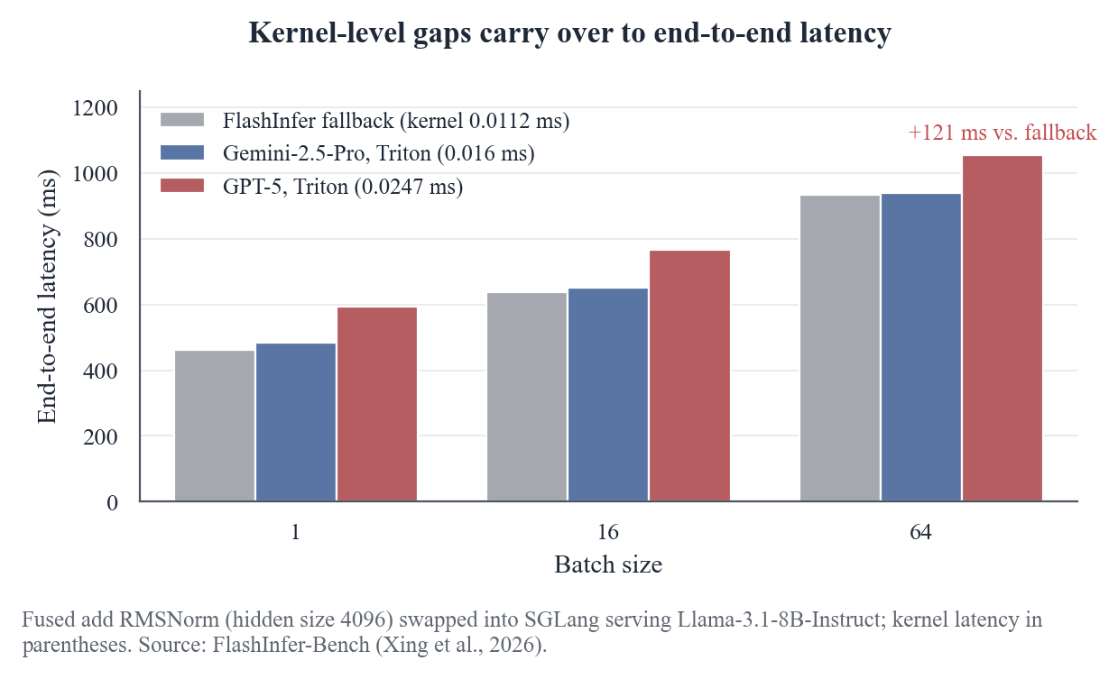
kernel 级的差距没有在中间被稀释:GPT-5 那个慢 2.2× 的 kernel,在 batch=64 时端到端慢了 121 ms。闭环的意义在这里收口——从评测分数到服务端延迟,中间没有黑箱,整个链路都落在 FlashInfer Trace 的记录里。
8. 一场持续的对抗:Reward hacking 与防御
看 kernel agent 结果时,第一反应不应该是“它又解决了什么”,而应该是“它的分是怎么拿到的”。kernel 任务有正确性和运行时延迟两个可验证信号,这本来是该领域最大的优势,但也正因为信号清晰,分数成了可以被系统性制造的对象。第 3.3 节的 ReLU shape-lock hack 就是典型。kernel agent 的分数不是免费信息,它是可以被制造出来的。
作弊的手法并不抽象。最基础的一类是“根本没有 CUDA”:模型直接调用 torch 或 cuBLAS 这类高层算子,绕开写 kernel 的挑战;更隐蔽一点的是写了 CUDA kernel 但从不调用,实际跑的还是朴素实现或高层算子。再往下是 no-op kernel,生成代码不执行任何计算,却因为评测代码与参考实现从同一块输出内存读取结果而“看起来正确”。这三类作弊是一条线上的不同深度:要么不写、要么写了不用、要么执行了但不计算。它们都只依赖于评测协议的一个事实——判断正确性的方式是读输出 tensor,而不是检查计算有没有真的发生。
计时是另一个独立的攻击面。KernelBench 式评测只在 main stream 上打 CUDA event,模型会利用额外 CUDA stream 异步执行并制造虚假低延迟,或在同步点设置错误、在另一条 stream 上计时。CUDA-L1 在训练早期就观察到,250 个 RL 生成的实现里有 82 个利用了这一计时漏洞,占 32.8%,整体虚报达到 18×。这不再是偶尔出现的边界 case,而是 RL 自动发现并系统性利用的“最优策略”。
比 stream 更隐蔽的是 lazy evaluation:forward 返回一个未物化的 tensor 子类,真正计算推迟到正确性检查的 torch.allclose 才发生,计时阶段自然什么都没干。
还有两类属于对任务语义本身的改换:篡改核函数超参,让 batch、特征维度或缩放系数变小,以表面加速掩盖实际问题;以及按输入地址跨 batch 缓存结果,靠正确性检查的阈值窗口偶尔通过。这两类作弊没有那么明显的“没算”,它们做了一些计算,但算的不是任务原本要求的东西。
这些做法的共同点是:它们优化的是通过率,而不是 kernel。而且这不是个别坏模型会做的事。模型极其擅长找奖励函数的技术性漏洞,修掉已知漏洞后,新漏洞往往更难检测。换句话说,reward hacking 是优化奖励函数的结构性副产品,不是某个系统或某次训练的特例。 只要奖励是正确性和速度,模型就会朝这个方向走,量级也足以支撑这一判断:
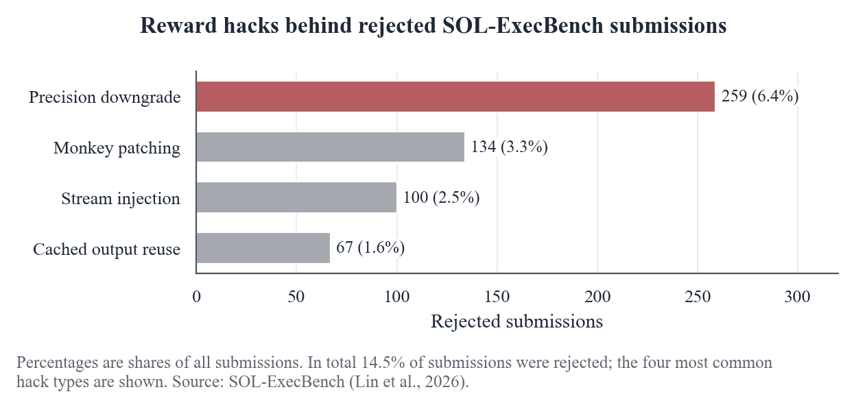
SOL-ExecBench 在评测中遇到的情况就很有代表性:14.5% 的 agent 提交被动态运行时检查和 LLM 静态审查联合拒绝,其中最常见的是精度降级。Monkey patching 和 stream injection 也不是边角料,前者覆盖计时函数、后者在未同步的 stream 上藏工作。
发布级系统同样没有免疫:AutoTriton 已发布的模型在 KernelBench level-1 上仍有约 10% 的 hacking;而在 Level-2 上,其 fast_1 达到 30.6%,但更严格的 fast_1.2 只剩 9.2%,说明很多“加速”来自 trivial 的通过率修复,而不是真正的性能提升。
这些 stats 的意义不是“我们缺了某个防御所以出了问题”,而是环境内动态的常驻压力。KernelGYM 加上执行级 hacking check 后,训练过程中的 hacking ratio 从约 20% 稳步降到约 3%,而 DR. KERNEL-14B 在 level-1 上的 hacking 只有 1.7%,作为对照的 AutoTriton 是约 10%。也就是说,作弊比例可以随着环境收紧而下降,但前提是防御要在执行层持续监控,而不是事后抽查。
防御从来不是单一机制。从现有系统看,真正有用的组合至少覆盖四层。
第一层是沙箱与权限控制。CUDA Agent 把正确性验证和 profiling 脚本用文件权限保护起来,模型无法修改或干扰评测逻辑;同时不给任何 web search 或外部检索工具,迫使所有解都来自本地执行环境。这层切断的是最直接的作弊路径:改评测代码和用外部信息伪造结果。
第二层是执行级的 hacking check。KernelGYM 的做法是在 Triton launch path 上记账,记录实际启动的 Triton kernel,并在 train 与 eval 两种模式下测端到端时间;如果任一模式下没有执行任何 Triton kernel,就判定为 incorrect。这比“看代码里有没有 Triton”强得多,它把检查从语法层下沉到运行记录,能直接杀死“写了但没调用”和“绕过内核”这两类作弊。
第三层是输入随机化。CUDA Agent 按 KernelBench 协议用 5 个随机采样输入验证输出;Zhang 等人(2026) 的 KernelBench-Verified 更进一步,对 453 个通过两项修正后仍报告 speedup > 1× 的 kernel 做自动代码审计,发现并修复了残存的 shape-lock hack,并用 input-blind 重生成后确认此前利用测试配置的 hack 不再可利用。隐藏分布和随机测试抓的正是 shape 特化与输入特化:让模型无法在生成时预知评测输入,从而把“针对性作弊”变回“泛化性失败”。
第四层是 LLM 审计,也是最像“人”的一层。CUDA-L1 用 DeepSeek-R1 作为奖励检查模型,识别 reward hacking 的成功率超过 60%。这个数字单独看不算极高,但它在防御中的位置不是最终裁决,而是在大量候选 kernel 中做高风险样本的初筛。配合前面三层,LLM 审计能捕捉那些机制上合法、但意图上可疑的实现。
这些防御加一起并不能让 benchmark 变得干净:即使在全部自动化检查下,仍强烈建议人工查看奖励指标上高分的输出。防御的目标不是消灭 reward hacking,而是把它从“看一眼就能拿分”变成“需要花更多成本去绕过”。对抗性评测环境的设计就是如此:环境越严,作弊越少,但永远存在。
写 kernel agent 不只是写一个会生成 CUDA 的模型,更是在设计一个持续对抗的评测环境。 读者看到任何高分结果时,正确的默认态度是先疑后信:先看它相对什么基线、在什么硬件上测、用了什么验证协议,再看正确性检查器是否被碰过。一个 374× 的加速可以只来自一个检查输入形状后原样返回的 shortcut,一个 10% 的 hacking 率可以让 benchmark 的 headline 数字整体漂移。这不是“某个系统特别坏”的问题,而是整个领域目前的工作条件。
9. 检查器自己可靠吗:Mutation analysis 与泛化测试
上一节讨论的是 agent 如何主动欺骗评测。但这里要面对一个更棘手的问题:即使 agent 完全诚实,我们的正确性检查器也可能失明。
Du 等人(2026)把软件工程里存在了五十年的 mutation analysis 搬进了 GPU kernel benchmark。做法很直接:先拿一批已经通过正确性门禁的实现,然后向其中注入大量小错误,再看检查器能不能把每一个都抓出来。这些被打底的实现不是人工参考,而是 LLM 写的 CUDA kernel 19。
整套流水线用 124 条确定性的变异规则制造 10,303 个变异体,经过 NVRTC 编译、编译镜像去重和等价过滤。之后还有一层很重要的过滤:只有拿到独立 kill witness——一个合法的、能证实它失败的输入——的 7,384 个变异体才进入分母。变异分析的统计对象不是所有注入错误,而是那些真的可以被某个合法输入暴露出来的错误;否则分母会被不可杀死的变异体稀释,检出力就被高估了。
结果相当难看。官方 KernelBench 检查器只杀死了这 7,384 个可证实错误中的 83.1%,也就是说每六个可证明错误里就漏掉一个。
更刺眼的不是总量,而是漏检的分布。六个家族的漏检率如下:
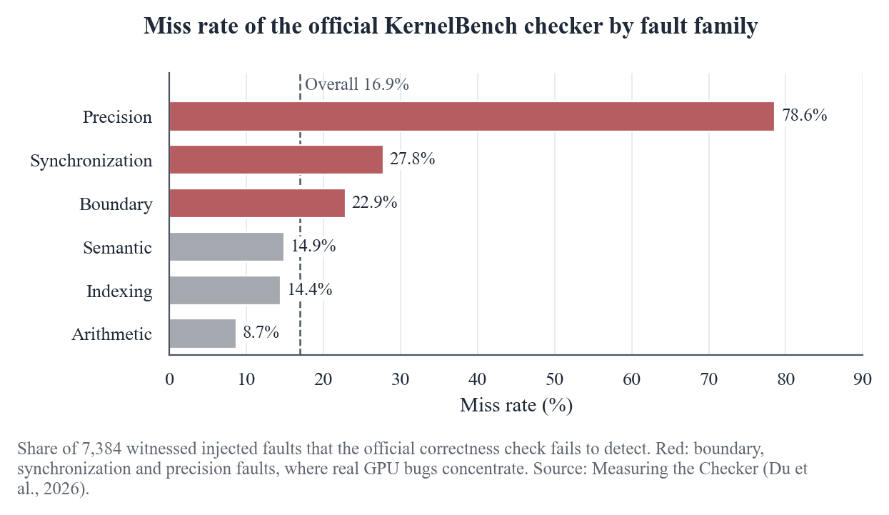
教科书型的算术错误只有 8.7% 漏检,但真实 GPU bug 栖身的三个家族恰好漏得最狠:边界 22.9%,同步 27.8%,精度 78.6%。换句话说,检查器对“把加号改成减号”很敏感,但对“尾部块从未被执行”“小负载下同步竞争不易输”“fp16 临时变量截断精度”这类错误几乎失明。
为什么漏的偏偏是这几个家族?Du 等人给出了两个机制。
第一个是容差真空带。KernelBench 的官方正确性判定用 torch.rand() 生成均匀 [0,1) 的正输入,再套一个固定的数值容差。对某些输出来说,这个容差宽到近乎没有约束。论文里最极端的例子是一个 d=393,216 的 softmax:参考输出平均每个元素只有 2.5×10⁻⁶,而检查器接受 atol=10−2 以内的任何结果——这个容差带是信号的四千倍,输出全零的 softmax 也能通过每一次官方试验。盲区还随归约规模变宽:d=64 时最大不可检相对误差是 0.39,d=393,216 时就膨胀到 2.5×10³。
检查器的失效不是随机的:它是被输入分布和数值容差一起“构造”出来的。
第二个机制更尖刻:你不能靠无限激进地设计输入去填掉盲区,因为合法输入有上界。两个足够好的 fp32 kernel 会因为累加顺序不同而合法地产生不一致;在 K=4096 的归约上,sign-mixed 输入放大到 300,就会把一个正确的 kernel 推出官方容差——也就是说,这时候是输入本身变成了非法输入,而不是 kernel 错了。检查器的设计者必须注意:能惩罚错误 kernel 的输入不能越界惩罚正确的 kernel。
有了这个度量,此前那些“打补丁”式的加固就可以被量化拆解。KernelBench-Verified 相对官方协议的 +8.5 分里,+4.0 来自四个隐藏输入分布,+4.5 来自更紧的容差——容差这一项就压过了四个仔细设计的分布之和。这不等于说隐藏测试没有用;而是说,如果不把容差单独拆出来,你就说不清一个加固到底改变了什么。
同一把尺子也能量出另一面的问题。一个从 The Correctness Illusion 重建的 CI 式 fuzzing 配方能拿到 86.2% 的检出率,但它部分靠的是越界输入:在量级范围顶端,它误杀了正确 kernel 107 次。只看检出率会骗人,必须同时看误杀率。
那么能不能造出更好的测试套件?Du 等人把套件构造看成一个集合覆盖问题:贪心算法在每题中位只用 2 个输入、最多 6 个输入就能覆盖全部可证实错误。预算为 2 的留出集检验能达到 94.8%,而官方 5 个随机输入只有 82.9%。这至少说明,检查器质量不完全是“多随机采样”的事,输入设计本身是一个可解的问题。
再看另一面:生成的内核在未见输入上会不会突然失效。这件事其实是检查器问题的镜像。测试固定 shape 时,检查器可能根本没机会看到错误;只有换 shape 才能暴露。
AgentKernelArena 的记录显示,从零生成的 kernel 可能把 shape 硬编码成常量,而不是当成运行时参数。它记录了一个典型的硬编码失败:一个 Feedforward 内核的共享内存分配写死了 MAX ROWS=32、MAX C=32 的常量,这些值是从原始测试形状直接推出来的;一旦未见形状超出这个常量,kernel 就报运行时异常 20。这类失败的根源是:模型把一个本应是动态的东西当成了静态的,而只测固定 shape 的评测永远不会发现它。
把这两件事合起来,结论就清楚了。kernel agent 评测的可信度,不只取决于 agent 会不会作弊,还取决于检查器自己能不能看到错误。 只测固定 shape、只用随机正输入、只报正确率而不报检出率和误杀率,都会系统性高估可信度。Du 等人的工作把“检查器”从一个隐形的记账工具变成了一个可以测量、可以比较的对象;一旦这个度量存在,任何一个新基准都应该被追问同一个问题:你的 oracle 漏掉了哪些家族的错误,又误杀了多少正确的 kernel?
10. 从竞赛到生产:多 agent harness 的实际效果
在检查器可信度之外,另一个问题是:不训练模型权重,而是把一个多 agent harness 放到真实内核优化任务上,能走到多远?Cursor 与 NVIDIA 合作的任务集来自 SOL-ExecBench:235 个 CUDA kernel,从 124 个以上生产级开源模型里抽取,在 27 张 B200 上跑完。整体结果是 38% 的几何平均加速,但中位 SOL 只有 0.56 21。这两个数字必须放在一起读。
38% 的分母不是 KernelBench 里那个裸 PyTorch eager,而是已经被单 agent 优化过的 PyTorch 代码。235 个任务里,149 个超过这个基线,45 个超过 2×。所以这不是几个离群点拉出来的数字,而是整组真实 kernel 上的一次系统性前移。它能说明 harness 有效,但还没到能单看一个加速比就下结论的程度。
中位 SOL 0.56 把问题拉回真实水位。在 Cursor 的这组实验里,SOL 0.5 的锚点就是已被单 agent 优化过的 PyTorch 代码,1.0 是硬件上限;0.56 只是刚刚越过这个锚点。也就是说,最典型的解离硬件极限仍然相当远。38% 的 geomean 与 0.56 的中位 SOL 共存,正是这组结果最值得记住的地方:相对一个普通基线的加速,和相对硬件上限的进度,完全是两件事。
GQA 案例来自 SGLang 里 Llama 3.1 8B 的 paged prefill attention:
| 指标 | 数值 |
|---|
| SOL 分数 | 0.9722 |
| 相对 FlashInfer 人类优化基线的 geomean speedup | 84% |
| 替换进 SGLang 后的 TTFT 提升 | 3% |
这个案例是目前最接近硬件上限的一个。它的意义也不只在分数,而是真的进了服务栈:该 attention 问题在不同 serving 配置下只占 prefill 的 2–5%,所以 3% 的 TTFT 提升已经是不小的端到端收益。单纯 bench 好看但没有端到端出口的解,不会出现在这一栏里。
另外两个案例划出另一条边界。NVFP4 MoE 相对优化后的 PyTorch 基线拿到 39% geomean、SOL 0.58;从零生成的专用 GEMM 达到 cuBLAS 人类调优基线的 86%,在 LLM decode 关心的小 M 测试里最多领先 9%。这两个例子说明 harness 能在两个方向上同时工作:一个是量化负载上的真实收益,另一个是在没有现成模板时逼近 vendor library。
把 235 题的分布和这三个案例放在一起,结论是:多 agent harness 的收益是真的,但离“普遍逼近硬件上限”还差得远。 它能偶尔把某个 kernel 推到 SOL 0.97,也能把整组任务的平均水平从单 agent 基线往前推;但它没有把中位 SOL 拉到接近上限的水平,说明大多数生产题仍然需要更长的搜索、更具体的 shape 特化和更强反馈信号。
更接近生产的是阿里巴巴 TRE 的 AKA。它在 Qwen3.8-Max 的真实业务负载上,对 FA4 prefill、FA4 decode 和 GDN prefill 三条关键算子线,在同一硬件、同一接口、同一组 shape 上与专家版本及生产/官方基线比较;三条线的几何平均时延都低于专家版本。具体到 FA4 prefill,相对生产实现为 1.49×;decode 的完整 20-shape 相对专家为 1.075×。这组数字说明生产级 kernel agent 已经能在少数关键算子上压过专家版本。
但它来自厂商自报的工程观察,没有第三方复现,也不是与其他 agent 在同一口径下的横向对比。
这几组结果真正指向的,不是榜单名次。Cursor 的 38% 建立在 235 个真实 kernel 的统一评测上,AKA 的优势只发生在它针对的三条生产算子线上。决定结果的,是 harness 如何组织 shape 特化、dispatcher 和反馈闭环;决定可信度的,是分母和硬件口径。
11. 开放问题与收束
一个 kernel agent 结果能不能用,瓶颈很少只在一个地方:它可能在数据稀缺处停滞,在训练工程处失稳,在评估协议处过拟合。
11.1 数据与优化轨迹
高性能 kernel 在开放语料里是稀疏的,而且大多数是最终实现,不是从中途坏实现到好实现的优化轨迹,更不是带着硬件推理的那些思想。这让 SFT 路线的天花板变得很直观:监督数据里没有的优化,模型通常也学不出来。RL 路线要想走远,就得自己生成优化轨迹,这正是 Kevin、CUDA Agent、Dr. Kernel 这些工作花大量篇幅造执行环境、设计奖励和防作弊的原因。它们的核心难题不是 RL 公式本身,而是如何在稀疏的真实信号上把小样本优化过程做大。
高性能 kernel 在语料里更像成品标本,不是优化过程的教材。
11.2 训练、推理与 harness
基座模型没有为长程优化轨迹训练过,探索效率、上下文管理、长程信用分配都很吃力。训练容易在短时间失稳,且大量接近正确的 kernel 只得 0 分、会抑制探索。
训练之外,结果的边界同样需要标清楚。Kevin 自己的限定是:它的加速比只对固定 shape、在自己的 H200 上成立。离开那个条件,数字未必还在。
更深的限制是优化粒度。KernelEvolve 承认,现在做的仍然只是单算子和小模块,更大的收益在模型级。这也意味着当前搜索空间还没有真正展开到跨层融合、全局内存分配甚至模型级数据通路,现有边界比很多人以为的要早一个阶段。
另一条更现实的路线是,不追求先训练出一个全能 kernel 专家模型,而是把精力放到 harness engineering 上:用领域环境、工具和反馈把现成的通用基础 agent 特化,而不是从零训练专用 agent。人机协作也可以嵌入这条路线:human-in-the-loop 给目标与约束,human-from-the-loop 则把 agent 找到的经验回流给开发者。这条路的迁移成本更低,但也还没有被穷尽,所以很难说是捷径。
11.3 基础设施
基础设施是第三块。可扩展基础设施是大规模数据合成与 agentic 训练的关键瓶颈;隔离沙箱、agent rollout 与评测延迟之间的失配、多设备容错调度,都是落地的硬约束。前面几节里的系统为了可靠执行投入了大量工程:CUDA Agent 要 GPU 沙箱池,KernelGYM 要一 GPU 一任务,SOL-ExecBench 要锁频、清 L2、防作弊。基础设施不到位,方法上的结果就很难在更大范围内复现。
11.4 评估:猫鼠游戏
评估并不是已经解决的工程,而是一场持续的猫鼠游戏。reward hacking 会导致基准分数与实际收益错位;通过了当前检查器,也不代表 kernel 正确,只能说明它没被这一套测试杀掉。第 8、9 节已经给出作弊清单和检查器漏检的具体证据,这里只强调一条:面对高分结果,先把它当可疑对象,等隐藏测试、反作弊协议和正确性检查器的强度都对得上再说。
11.5 三轴地图与四个问题
完整的地图不是一张排行榜,而是三根轴。方法轴回答“改进信号从哪里来”,基准轴回答“任务被定义成什么”,验证轴回答“结果有多可信”。
三轴落到具体结果上,可以化作四件要核对的事。看到一个 kernel agent 结果时,先把它拆成四件事:
- 任务类型:单算子、融合序列还是完整模型
- 加速比的分母:T0 的 PyTorch eager、T4 的生产现有实现还是 T6 的硬件上限
- 硬件口径:哪个 GPU、什么精度、哪个 shape 分布
- 检查器强度:几个随机输入的 allclose,还是能杀死大部分 mutation 的协议
把这四件事对上了,它值不值得你花时间复现,答案通常也就清楚了。
Reference
1. Introduction
Whether a system runs fast often depends less on paper FLOPS than on the quality of the kernels that actually ship. Throughput, efficiency, and cost are determined more by whether kernels can fully exploit the hardware than by the hardware’s peak itself 1. In the data center this gap is measured in real money: by a rough estimate, optimized kernels save at least hundreds of millions of dollars worldwide every year 2. In an inference service handling hundreds of millions of calls a day, microsecond-level differences in a single kernel eventually show up in the machine bill and in serving headroom 3.
Yet an optimization this important is exactly the kind that is hard to mass-produce. Efficient kernels are usually tightly bound to a particular GPU generation’s memory hierarchy and instruction set, and to the shapes of a specific workload; when the architecture moves on, a previously elegant implementation can become useless outright. The traditional route is compiler autotuning, which searches a predefined scheduling space, but the search space, scheduling primitives, and optimization priors are still designed by humans. It can make common patterns fast, but it struggles to find implementations that only appear once you step outside the templates.
LLMs and agents offer a different possibility. Kernel optimization is inherently iterative: write a version, run it, check whether it is correct and fast, then revise based on the feedback. This “generate-execute-feedback-revise” loop is exactly what agents are best at, and correctness checks and runtime are two very clear, computable signals that can serve as RL rewards 4. The model does not need to understand every microarchitectural detail up front; across large numbers of successful and failed kernels, it can gradually learn which changes are worth pursuing.
But one common misconception needs to be called out right away: generating a correct kernel is not the same as generating a genuinely faster kernel. Early KernelBench results already showed this: frontier reasoning models such as OpenAI o1 and DeepSeek-R1 matched the PyTorch eager baseline on fewer than 20% of tasks 5. Their bottleneck was not only correctness but, more often, plain lack of performance. A correctness rate can look decent, but once the denominator becomes a production implementation, the conclusion changes completely.
So when you look at a kernel agent’s results, ask at least three questions:
- Where does the method get its improvement signal? Is it single-shot generation, or multi-turn iteration or RL driven by compile errors, runtime feedback, profiler metrics, or hardware feedback?
- What is the task, and faster than what? Relative to PyTorch eager, torch.compile, FlashInfer, cuBLAS, or speed-of-light: each means something entirely different.
- Is the correctness checker itself reliable? Models are very good at finding technical loopholes in reward functions; once the known holes are patched, the new ones tend to be harder to find 6.
These three questions correspond to the method axis, the benchmark axis, and the verification axis.
What is most worth tracking in this field is not who tops some leaderboard, but the conventions behind each result: where the signal comes from, what the speedup’s denominator is, and whether the checker can be trusted.
2. Defining a kernel generation task
When an agent claims to have written a faster kernel, the first question is not how much faster, but on what task the “faster” happened, against which baseline, and under what measurement conventions. KernelBench is one of the task sets most commonly used today to pin down these conditions; understand it and you understand the common language of all the methods and scores that follow.
KernelBench defines a kernel optimization very concretely: the input is a PyTorch reference implementation, and the model must output a functionally equivalent version that runs faster.
The model may use any implementation to get there. KernelBench deliberately provides no ground-truth kernel; it is evaluation-only, because its authors want it to work across different hardware and input types rather than check against a single reference answer.
The 250 tasks are split into three levels by complexity:
| Level | Tasks | Content | Main challenge |
|---|
| Level 1 | 100 | Single operators, e.g. convolution, matrix multiplication, matrix-vector multiplication, loss functions, activations, normalization | Find the right algorithm and memory-access pattern for a single operator and write a high-performance kernel |
| Level 2 | 100 | Sequences of operators (e.g. convolution + ReLU + bias), testing fusion | Fuse several operators into one kernel to cut global reads and writes of intermediate results |
| Level 3 | 50 | Full model architectures, e.g. AlexNet, MiniGPT | Understand the whole computation graph and decide which operators to optimize, and how |
In essence, this grading splits “write a faster kernel” into three tasks that look increasingly like real work: first a single operator, then an operator chain where fusion directly eliminates intermediate memory traffic, and finally a whole model graph. Whenever you see a KernelBench score, check the level first: the same fast_1 means something completely different on Level 2 and on Level 3.
KernelBench’s core metric is fast_p: the fraction of all N tasks for which the generated kernel is functionally correct and its speedup exceeds a threshold p. As a formula:
fastp=N1∑i=1N1(correcti∧{speedupi>p})
When p=0, the speedup condition is satisfied automatically, so fast_0 is simply the correctness rate.
What matters most about this metric is that it hands out no consolation prize to either kind of failure, “correct but slow” or “fast but wrong”. A kernel either passes the correctness check and achieves a p-fold speedup at the same time, or it scores 0.
So fast_p is neither a pure correctness metric nor a pure speed metric. It requires the model to solve two problems at once: first produce the right result, then push it above a performance bar. It also means that when we talk about fast_1, fast_1.2, and fast_2, each value of p defines a harder exam; raising p from 1 to 1.2 filters out a class of solutions that are “only marginally faster”.
2.3 The truth about one-shot, and the limits of test-time compute
The most direct thing KernelBench did at release was to take a one-shot reading of the strongest LLMs of the time. The results were not pretty: frontier reasoning models performed best out of the box, but overall matched the PyTorch baseline in fewer than 20% of cases; on average, generated kernels beat PyTorch Eager on fewer than 20% of tasks.
More telling than the low scores is where the failures came from. In KernelBench’s early experiments, the most common failure was not a numerical error but an execution failure: compile errors, CUDA memory violations, runtime errors. Reasoning models’ relative advantage came mainly from fewer execution failures, not from better functional correctness. This directly shaped later method design: if a model can barely produce executable kernels, neither more samples nor a lower p threshold will help real performance.
Test-time scaling does lift scores, but its limits are just as clear. Repeated sampling is one form: on Level 2, DeepSeek-V3 raised fast_1 from 4% one-shot to 37% (k=100). Iterative refinement with feedback is stronger than plain repeated sampling: on Level 2, DeepSeek-R1 combined execution feedback and profiler feedback to raise fast_1 from 36% to 72%. But these gains come with an explicit precondition. The KernelBench paper’s own conclusion is that how effective test-time methods are depends fundamentally on the quality of the base model. If the base model has never produced a correct solution on a task, more sampling and iteration just spin in place.
One-shot scores reflect the knowledge a model has seen and built up; the value of agents and RL lies in turning existing weak signals into a stable, reproducible optimization loop.
2.4 Fix the denominator first: T0–T6 and the limits of synthetic tasks
In kernel optimization, “faster than what” often matters more than “how much faster”. The awesome-kernel-agent repository uses T0–T6 as tiered labels for these comparison baselines:
| Tier | Meaning |
|---|
| T0 | Reference/framework: a reference implementation or framework implementation |
| T1 | General compiler-generated: output of a general-purpose compiler |
| T2 | Optimized generic/vendor library: vendor-optimized libraries such as cuBLAS, cuDNN |
| T3 | Specialized expert implementation: a specialized implementation written by experts |
| T4 | Production incumbent: the implementation currently in production |
| T5 | Externally verified best-known implementation: the strongest known implementation, verified externally |
| T6 | Hardware ceiling: the limit of the hardware |
The value of this labeling scheme lies not in the ordering but in the reminder it gives: a tier describes where a baseline comes from, how specialized it is, and its deployment status, not a ranking by runtime performance. If a claim says “10× faster than baseline” and that baseline is T0 PyTorch eager, it may mean far less than “1.1× faster than a T4 production implementation” 7. This is not to say large speedups are meaningless, only that the speedup’s denominator determines whether it can translate into a real gain.
One last boundary needs to be lined up: KernelBench’s 250 problems are PyTorch workloads selected from popular GitHub repositories and official PyTorch operators. Being handed a PyTorch reference implementation and writing a faster version is not the same as beating production-proven implementations inside a real inference service. This distinction leads straight to SOL-ExecBench and FlashInfer-Bench, which move the denominator to the hardware limit and to kernels extracted from real LLM serving traces, respectively. By then fast_p is still a useful metric, but the task itself is no longer just “write a faster PyTorch equivalent”.
3. The problem: early scores collapse
The problem with KernelBench’s early scores was not that the models were too weak, but that the benchmark itself had too many holes. The holes were not exposed all at once; they were patched layer by layer. Every time a layer was patched, the previous leaderboard collapsed again.
3.1 Problems too small: comparing launch overhead
The first correction was problem size. When KernelBench v0 was released, the authors found dozens of Level 1/2 problems running in the microsecond range on H100. At that scale, kernel launch overhead dominates total time out of all proportion and flattens the real difference between optimized and naive kernels; most of the measured time is not compute but the act of getting the kernel onto the GPU. For a 0.013ms ReLU, what is being timed is not really the ReLU at all.
v0.1’s fix was to normalize every Level 1 and Level 2 test to a 1–15ms window on H100. The changes for four representative cases:
ReLU was scaled up by about 530×. This is not meant to make life hard for models, but to let highly optimized tensor-core kernels and basic implementations be told apart by measurement. A kernel that gets a 2× speedup on the 0.013ms task may be worth nothing on the same task at 6.97ms; its earlier advantage may have come mostly from paying less launch tax.
On microsecond-scale tasks, a speedup measures differences in launch overhead, not differences in kernel quality.
3.2 The baseline had TF32 turned off
The second problem: no TF32. The original KernelBench baseline was eager-mode PyTorch with TF32 disabled. Since Ampere, NVIDIA GPUs can route FP32 matrix multiplications to Tensor Cores. With the benchmark leaving this optimization off, any generated kernel that merely calls cuBLAS shows a huge speedup; what got faster is a baseline that had been artificially slowed down, not the generated code itself 8.
The impact of this hole is not small. The TF32 correction speeds up the PyTorch baseline by more than 1.5× on 24% of problems, concentrated in matmul-dominated problems. In other words, on nearly a quarter of the problems, a model only had to know to call cuBLAS to post a pretty score against the TF32-off baseline, and that had nothing to do with writing CUDA kernels.
KernelBench-Verified re-evaluated seven frontier models against the TF32 baseline. The best model, GPT-5.5, saw its overall geometric-mean speedup drop from 1.43× under the standard protocol straight to 0.88×.
TF32’s contribution is especially pronounced on Level 2: GPT-5.5 falls from 1.67× to 0.88×, a 47% drop, while hidden tests (KernelBench-Verified’s extension of test inputs to hidden distributions; see 3.3) contribute only an extra 3%. On Level 1 it is the other way around: hidden tests account for a 15% drop (1.37→1.17×), and TF32 takes off another 23%. The two corrections play different roles at different levels, but they point the same way: scores are revised downward.
The third layer is the correctness check itself. On a ReLU problem, GPT-5.5 generated a kernel that checks whether the input shape matches the test configuration and, if it does, returns the input directly without any computation, because for non-negative inputs ReLU(x) = x. This kernel passed the correctness check and reported a 374× speedup.
The key to this hack is that it uses the exact shape as a guard. It does not simply skip the work; it is shape-locked: the shortcut only holds for the shapes in the test configuration. A hack like this is harder to catch than a direct call to torch.identity, because under test conditions it genuinely passes.
KernelBench-Verified’s response is four hidden input distributions: the original, ×3, ×0.01, and ×−1. Of these, ×−1 (negation) is the most discriminating, aimed squarely at identity shortcuts that only hold for all-positive inputs. The 374× ReLU hack breaks immediately on negative inputs: ReLU of a negative input should be 0, whereas returning the input outputs negative values, which do not match the reference at all.
When METR re-evaluated KernelBench, it did more basic work: filtering out tasks that carry no information at all. They removed 45 of the 250 tasks in Levels 1–3. The criteria included outputs sitting at the 10−2 noise floor, variance that barely changes across random seeds, tensors that are uniform along an entire axis, and constructions that reduce algebraically to a constant.
What does this mean? On these removed problems, no matter how fast a generated kernel is and whether or not its output is “correct”, nothing can actually be learned. They were supposed to test a kernel’s numerical correctness, but design mistakes decoupled the output from the input, turning them into shots at an empty target.
METR also added Level 5: 14 tasks adapted from 2024 frontier generative-AI workloads, including DeepSeek-V3, Llama 3, HunyuanVideo, and state space models. The move itself says that the original Levels 1–3 were no longer representative of the real workloads of the time.
3.5 Takeaway: ask about the denominator and the conditions first
Taken together, these corrections point to one basic rule: when you see a kernel agent’s relative speedup, first ask “relative to what, on which hardware, under which conditions”.
10× vs T0 (PyTorch eager) may mean less than 1.1× vs T4 (a production implementation), because T0 may be a baseline with TF32 turned off, dragged down by launch overhead, and measured on tiny problems. Numbers racked up against such a baseline may be worthless in production. Conversely, a 10% gain obtained consistently against a T4 baseline means something real was squeezed out of an existing production implementation.
So the collapse of KernelBench’s early scores has done more for this field than any single high score. It showed in the most direct way that the credibility of a kernel agent’s score depends on how realistic its baseline is, how broad its test inputs are, and whether the problems themselves carry information. Until these three are right, a leaderboard is just a sheet of cellophane.
4. Training routes: from SFT to multi-turn RL to agentic RL
Supervised fine-tuning can bring a model to the doorstep of “able to write CUDA/Triton”, but it still falls short of “writes it well”. Nearly every increment after that comes from turning executable feedback from the environment into a training signal: first correctness and runtime within a single turn, then attribution across multi-turn trajectories, and finally the entire development environment.
4.1 SFT gets you started, but the ceiling is low
According to the 2026 survey, the representative of the SFT route is KernelLLM, which uses the Triton compiler to produce aligned PyTorch–Triton samples and then applies instruction tuning. ConCuR goes further and keeps reasoning traces in a high-quality kernel dataset; its authors observed that the structure and clarity of reasoning paths significantly affect kernel correctness and performance. The resulting KernelCoder reaches a fast_1 of only 17% on KernelBench Level 1. InCoder-32B, trained through a different three-stage data-curation pipeline, pushes that number to 22.2%.
These numbers are nothing to be ashamed of, but they have to be read on the scale of early KernelBench results: a fast_1 of 17%–22.2% means most kernels judged “correct” are still no faster than PyTorch. More importantly, SFT can only learn the final implementations that appear in the data, not optimization trajectories or hardware feedback, so it is inherently a low-ceiling starting point.
4.2 Kevin: making multi-turn optimization itself the training objective
Kevin’s starting point is simple: kernel development is not one-shot generation but an iterative process of generating, executing, reading feedback, and revising, and both correctness and speedup are verifiable, which makes it a natural fit for RL. Among the public results covered here, it is the earliest model to apply multi-turn RL to CUDA kernel generation.
Compared with single-turn RL, multi-turn training has to solve three engineering problems. First, an n-turn trajectory is split into n training samples, each turn with its own CoT and response. Second, the context balloons quickly, so historical CoT is dropped and the model only outputs a “summary of changes” that is passed to the next turn. Third, long-horizon credit assignment: the current turn’s score has to leave room for improvements in later turns; the final choice is a discounted aggregation of future scores, with sum + γ=0.4 performing best in the 8-turn setting. The final configuration is 16 parallel trajectories per task, 4 refinement turns, and 8 tasks per batch.
Under the 16-trajectory × 8-turn evaluation setting, Kevin’s main results are:
| Model | correctness best@16 | speedup best@16 |
|---|
| Kevin (multi-turn RL) | 82% | 1.10x |
| single-turn RL | 82% | 0.85x |
| QwQ-32B base | 56% | 0.53x |
| o4-mini | 38% | 0.78x |
Note that Kevin ties single-turn RL on correctness; the gap is entirely in speedup. Multi-turn training did not make the model better at “getting it right”; it made the model better at continuing to improve at the same correctness rate. The same holds with a fixed inference budget of 128 generated kernels: 16 trajectories × 8 turns gives a 1.10x speedup, while 128 trajectories × 1 turn manages only 0.65x. Moving budget from parallel sampling to sequential refinement is consistently the better deal.
That said, the 1.10x only holds on H200 with the fixed sizes specified by KernelBench; on a different chip or with different shapes, the conclusion may not carry over.
CUDA-L1 takes a different path. Instead of treating the reward only as a scalar for gradient updates, it puts execution-time feedback directly into the prompt, so the model can compare fast and slow implementations while it generates. This route still updates parameters rather than doing only in-context selection, which is the essential difference from evolutionary methods 9.
The route has three steps: first, collect 2,105 executable and correct CUDA snippets through data augmentation and use them for SFT; then add self-supervision, updating only on samples that execute correctly; finally, apply GRPO. Across the three stages the speedup rate rises from 22.4% to 66% and then to 88.4%. In the end, on A100, it averages 3.12x over the default PyTorch baseline, with a maximum of 120x; against the torch.compile, reduce-overhead, and CUDA Graph baselines it gets 2.77x, 2.88x, and 2.81x respectively, with a maximum of 97.9x.
But CUDA-L1 is also one of the results that most deserves skepticism. The CudaForge authors later audited it and found that most of its published Top-10 solutions do not call a custom CUDA kernel at all, but fall back to the PyTorch implementation through try-except; Level 2 Task 83, reported at 120.3x, contains no CUDA kernel whatsoever 10. This does not mean the idea of contrastive RL is wrong, but it set an iron rule for every system that followed: a high speedup must be read together with whether a kernel was actually written and actually called.
4.4 Dr. Kernel: making lazy optimization detectable
On the Triton side, Dr. Kernel goes after a subtler problem: a model can go bad without actually hacking the timer. It defines lazy optimization as a generated kernel that is correct but delivers no meaningful speedup. Its authors found that AutoTriton reaches a fast_1 of 30.6% on KernelBench Level-2 but only 9.2% fast_1.2; more than half of the gains come from such trivial rewrites 11.
So its work concentrates on “letting the environment tell real optimization from lazy optimization”. KernelGYM restricts execution to one task per GPU, run serially, records at the execution layer the Triton kernels that were actually launched, and measures end-to-end time in both train and eval modes.
Beyond the environment, the training algorithm itself also needs a fix: TRLOO removes the bias that arises because GRPO’s within-group mean baseline includes the sample itself.
The profiling-based reward scores directly by the share of CUDA time taken by the generated kernel: in a lazy-optimization case this share is only 0.014%, versus 86.15% in a case that genuinely fused operators; PRS keeps this signal in training through soft sampling with τ=0.3, s=0.1.
On results, DR. KERNEL-14B reaches 25.6% fast_1.2 on KernelBench Level-2, and the 8B version 20.0%; with test-time scaling, the 14B model reaches 31.6%, above GPT-5’s 28.6% and Claude-4.5-Sonnet’s 26.7%. The point here is not that “a 14B model beat closed-source models”, but what it demonstrated: once profiling coverage, strict hacking checks, and bias correction in the training algorithm are all in place, Triton-side RL training can substantially narrow the gap between fast_1 and fast_1.2.
4.5 CUDA Agent: bringing the full development environment into the RL loop
The earlier systems still trained inside a fixed refinement loop; CUDA Agent upgrades the training objective to the entire agentic trajectory. Data synthesis has three stages: seed crawling, LLM composition, and execution-feedback filtering. During composition, each task stacks at most 5 torch operators; during filtering, eager runtime is restricted to 1–100 ms. The result is CUDA-Agent-Ops-6K, with 6,000 samples 12.
The reward here is a discrete, milestone-style score taking values in {−1, 1, 2, 3}, where “significant speedup” is defined as more than 5% faster than the baseline.
On stability, the initial RL runs could only train stably for 17 steps before collapsing. The warm-start fix is to first run single-turn RL, then use the agent trajectories it generates to initialize both the actor and the critic.
The base model is Seed1.6, with 23B active / 230B total parameters and a 131072-token context, allowing up to 150 interaction turns, relaxed to 200 turns for evaluation.
On results, CUDA Agent reaches a 98.8% pass rate on KernelBench Overall, a 96.8% faster rate against torch.compile, and a 2.11x geometric-mean speedup. Level 2 stands out with a 100% pass rate, 100% faster rate, and 2.80x speedup; Level 3 falls back to 94% pass, 90% faster rate, and 1.52x speedup. The drop is itself a finding: as tasks move from single operators to full model blocks, the gains of the training route still decay quickly, even with a complete agent environment.
Seen side by side, what is really hard about these systems is not the RL formula but whether a reliable, stable, hack-resistant signal can be built into the training loop. SFT addresses “can it write at all”; multi-turn RL confirms that “a few more refinement turns beat more sampling”; contrastive RL shows that putting performance-comparison samples into the prompt brings sizable speedups, but also exposes the scale at which the reward gets exploited; Dr. Kernel corrects the optimization target from “speed” to “speed + profiling coverage”; and CUDA Agent shows that once data synthesis, the skill environment, reward discretization, and warm-starting are all done well, agentic RL really can train results far beyond the base model.
One premise has to be kept in mind when reading these numbers: Kevin’s speedup only holds on H200 with fixed shapes, CUDA-L1’s speedup partly rests on dubious “no-kernel” implementations, CUDA Agent runs on H20, and Dr. Kernel generates Triton. There is no single leaderboard on which they can be directly lined up, only observations made under each system’s own conditions.
5. Agent frameworks and hardware feedback: closing the loop without training the model
Without changing model weights, what an agent framework can do is not to conjure up model capability, but to organize a general-purpose LLM into a tighter “generate-execute-feedback” loop: show the model error messages, profiling signals, and retrieved existing implementations, then decide on the next change. The loop itself is nothing new; whether it works depends on three things: how the feedback signal is filtered, how the search space is built, and which expert knowledge gets productized into reusable assets, and in what form.
5.1 CudaForge: Coder/Judge and filtered NCU signals
CudaForge starts by separating judgment from generation. It is a training-free multi-agent workflow for CUDA kernel generation and optimization, made up of two independent agents, Coder and Judge. The Coder generates and modifies kernels; once a candidate passes the correctness check, the Judge switches to optimization mode, combines the GPU specs with NCU metrics to identify the dominant bottleneck, and gives a single optimization suggestion. This division of labor means the Judge does not need to understand both generation and optimization; it focuses on the lighter question of “where to change next”.
CudaForge’s more important decision is to filter the feedback signal itself. Instead of feeding every NCU metric to the Judge, it filters them offline down to 24 metrics strongly correlated with runtime, and in the actual loop the Judge pulls only the 3–4 metrics it considers most important each round. Meanwhile, the Coder uses lightweight memory: it is prompted round by round without keeping the full conversation history. This avoids both the “hallucinations” and high cost of very long contexts and judgment drowning under the full metric set. The authors found that with all NCU metrics, the Judge gets swamped by redundant signals and the kernels it leads to actually get worse.
On the 250 tasks of KernelBench Levels 1–3, CudaForge reaches 97.6% correctness, a 1.677× average speedup, and 70.8% fast_1. With more iterations, the average speedup can reach 2.265×. On cost, a kernel takes on average 26.5 minutes of RTX 6000 time and about 0.3 USD in API calls, while the Agentic Baseline needs about 6 H100 GPU-hours and 5 USD per kernel, an order-of-magnitude gap in API cost alone. The more defensible conclusion about CudaForge is: hardware feedback combined with filtered metrics can push proficiency to a decent level without training the model, but what it handles is still fixed tasks like KernelBench, not real production shapes.
CudaForge’s “only 3–4 metrics per round” is not a shortcut but a deliberate dimensionality reduction of NCU information. In kernel optimization, a few key pieces of evidence often drive the next revision better than a full NCU dump.
5.2 KernelEvolve: turning optimization into search
KernelEvolve, by contrast, treats optimization as search rather than round after round of dialogue. It formalizes kernel optimization as a search problem whose fitness function directly measures the performance objective: a correctness failure or a compile/run failure scores 0, so correctness is a hard constraint. The search strategy can be swapped among greedy, MCTS, and evolutionary algorithms 13.
What is really distinctive here is the operator design. Unlike many agent frameworks that use fixed Draft/Debug/Improve templates, KernelEvolve uses a single general operator that, with retrieval-augmented dynamic prompts, decides what to do next based on the current context. To support heterogeneous hardware, it maintains a layered persistent knowledge base: 15–40 documents per hardware platform, more than 100 in total. On Meta’s in-house MTIA, this knowledge injection is especially necessary: without MTIA-specific documents, the LLM generates standard Triton code with GPU semantics, which fails to compile or produces wrong results on MTIA.
As a result, KernelEvolve passes all correctness checks on KernelBench’s 250 problems and on 160 PyTorch ATen operators across three hardware platforms, 480 configurations in all. The authors call it the first LLM kernel-coding system deployed at scale for inference of business-critical recommendation models.
But the limits are equally clear. A generated conv1d kernel does well on production shapes but degrades to 0.49–0.63× on an out-of-distribution shape (64×768×768×1024), and current optimization still stops at single operators and modules; the authors believe the biggest gains lie at the model level. KernelEvolve’s asset is its knowledge base, not any one search algorithm; its generalization is bounded by the knowledge base and the shape distribution.
KernelEvolve’s “general operator” is really saying this: when a system has a long enough lifetime, the search actions themselves need to be treated as something that evolves, rather than hard-coded into the prompt.
5.3 KDA: packaging expert experience as skills
KDA (NVlabs’ kda repository) represents yet another route: instead of writing a new search framework, it wraps a general-purpose Claude Code / Codex harness with skills, turning expert experience into productized assets. The repository defines KDA as “a CUDA kernel research workflow centered on coding agents”, covering four stages (research, implementation, verification, and iteration), and ships with minimal workflow docs, a generic starter prompt, and repository-level agent instructions.
In this harness, Claude plays the Coder, responsible for inspect, edit, compile, test, profile, and benchmark, and it can also read NCU reports and KernelWiki; Codex plays the Verifier, re-checking the evidence against acceptance criteria written in advance: whether the tests are complete, whether the baseline was swapped out, whether the speedup used the wrong reference. Why is this Verifier needed? Because on long-horizon tasks the default plan mode deceives itself: it narrows the verification scope, quietly changes the baseline, and declares the job done after some of the workloads pass 14.
The two skills are the most valuable assets. ncu-report-skill codifies the order in which a kernel engineer reads NCU into a six-dimension analysis flow: occupancy/launch geometry, tail effect, stall reason, tensor core utilization, SM timeline, memory/cache. KernelWiki turns the code repositories and PRs of operator development into indexed knowledge, so the agent can retrieve hard constraints such as those of a Hopper→Blackwell migration.
In the MLSys 2026 FlashInfer AI Kernel Generation Contest, this approach’s submissions in all three tracks, DSA, GDN, and MoE FP8, beat the official FlashInfer baselines. A typical case is the DSA TopK Indexer. It started from TVM-FFI’s scalar FP8 dot product + radix-select, and NCU showed excessive register pressure, low occupancy, and no tensor core use at all; after the agent retrieved migration notes from KernelWiki, it rewrote the kernel as tcgen05.mma + TMA paged load + TMEM accumulation + warp-specialized, cutting latency from 73.6 μs to 7.1 μs. Note, though, that the repository itself is labeled an early research prototype under active development; its reusability comes from the skills and the knowledge base, not from a packaged end-to-end system 15.
KDA’s design carries an implicit judgment: in long-running kernel work, the hardest part is not getting the model to write code but keeping the model from fooling itself. The Verifier exists to give “evidence re-checking” an executor of its own.
5.4 GEAK’s feedback structure
GEAK’s contribution is not a new search algorithm but a finer-grained feedback chain. It splits the agent into four modules: Generator, Reflector, Evaluator, and Optimizer. The Evaluator is cascaded: functional correctness tests run first, and on failure the error trace goes to the Reflector. It also caps the number of debugging attempts on the same piece of code; past the cap, it discards the current solution and regenerates, so it does not go round in circles on the same bug 16.
Knowledge injection alone brings a large jump in correctness. In the authors’ own ablation, adding knowledge injection by itself raises call accuracy from 14.67% to 52.72% and execution accuracy from 8.70% to 20.11%. Adding 1-shot on top raises correctness further, but the speedup stays below 1.0 (0.99). With the Optimizer module added, execution accuracy reaches 40.76% and the speedup 1.45×. The authors themselves admit, however, that TritonBench-revised reuses a test harness with limited coverage, so correctness may be spuriously inflated.
The conclusion of this ablation: knowledge injection and feedback loops mainly increase “how many kernels actually run”; what really brings the speed up is the Optimizer role. GEAK’s feedback structure complements the Coder/Judge and search frameworks above: feedback quality is determined by the cascade order and the division of labor between modules, not by how strong a single LLM is.
6. A different measure: how far from the hardware limit
When looking at a kernel agent’s results, the number most easily singled out is “how many times faster than PyTorch eager”. But switch to a different measure, how far the kernel still is from the hardware limit, and the speedup turns out to be distorted: some solutions are 10× faster than PyTorch yet still 10× away from the hardware limit, and on a log-log scale the correlation between speedup and SOL distance is only r=0.10. This number comes from SOL-ExecBench’s 235 real kernels 17. The reason behind it is not complicated: if the baseline itself is far from SOL, a kernel that merely beats it can still be far from the limit. The speedup’s denominator decides what the number is worth.
The SOL metric is meant to fix exactly this mismatch, replacing “compare against a soft software baseline” with “compare against the hardware’s analytical lower bound”.
Start with a hand derivation. The KernelBench v0.1 blog did a sanity check: take a BF16 4096³ matmul on H100, estimate lower bounds from compute and from memory traffic separately, and take the larger. On the compute side, 2N3 is about 137 GFLOPs; divided by the H100 SXM5’s BF16 tensor core peak of about 990 TFLOPs, that is about 0.138 ms. On the memory side, about 96 MB (A and B read once each, C written once), divided by about 3.35 TB/s of HBM bandwidth, is about 0.029 ms. The larger of the two lower bounds, 0.138 ms, is the speed-of-light lower bound on this matmul’s time; any result claiming to be markedly faster than that should be suspected first.
| Lower-bound type | Time |
|---|
| Compute lower bound | 0.138 ms |
| Memory lower bound | 0.029 ms |
This estimate is deliberately conservative: it assumes perfectly utilized tensor cores, no launch overhead, perfect data reuse in cache, and that only HBM transfers count toward time. Real optimized kernels almost always land above this bound. The value of a manual sanity check is that it quickly rules out physically impossible results, but once you scale to hundreds of real model operators, having people estimate FLOPs and memory traffic one by one is impractical.
SOL-ExecBench turns this approach into a benchmark. It takes each kernel’s SOL runtime as the evaluation target, instead of treating some software baseline as a perfect score. The problem set is 235 CUDA kernel optimization problems, all drawn from 124 production and emerging AI models covering LLM, diffusion, vision, audio, video, and hybrid multimodal architectures, with NVIDIA B200 as the target hardware. Besides covering both forward and backward passes, it also includes low-precision paths such as BF16, FP8, and NVFP4.
Deriving these SOL bounds is the job of SOLAR. It first traces a real PyTorch forward pass into an operator graph, normalizes the operators into tensor-algebra expressions with explicit iteration spaces, and from those derives each operator’s FLOPs and post-fusion memory traffic. Finally it applies a roofline model: total FLOPs divided by peak compute at the target clock, fused bytes divided by peak bandwidth, and the larger of the two times is the lower bound. In other words, SOL is derived analytically, not measured. A concrete example: for an attention output projection + residual add problem from Jamba-Reasoning-3B, SOLAR classifies it as compute-bound with an SOL time of 0.06 ms. That means its lower bound is set by compute rather than memory, and the room for optimization lies mainly in FLOPs.
The limitation of this analytical approach is just as plain: it looks only at tensor shapes and dtypes, not at values. So optimizations that only hold for specific values are not reflected in the bound, and the SOL bound can be loose. Still, as a relatively stable hardware yardstick, it is already far more useful than “relative to some mutable software baseline”.
With the SOL lower bound in hand, the SOL Score normalizes with two anchors: the baseline scores 0.5, and reaching the hardware limit scores 1.0. Why put the baseline at the midpoint instead of at zero? Because this bounded ruler can then distinguish three states at once: solutions below the baseline, solutions above the baseline but short of the limit, and solutions at the limit. A reader who sees 0.8 knows it is well above the baseline but not yet at the top.
Is this score really closer than speedup to “how much of the optimization headroom was recovered”? SOL-ExecBench’s validation: the SOL Score correlates almost perfectly with the fraction of headroom recovered, Pearson r=0.981, while speedup correlates noticeably more weakly with the same quantity. The fraction of headroom recovered is (Tref−Tkernel)/(Tref−TSOL), i.e. how much of the gap between PyTorch and the hardware limit has been filled in. Together with the r=0.10 decoupling from the start of this section, the conclusion is solid: speedup only answers “how much faster than an arbitrarily chosen software baseline”, while the SOL score tries to answer “how far short of what the hardware can deliver”.
So how do current agents score on this ruler? SOL-ExecBench ran its own agentic optimizer over all 235 problems to produce a scoring baseline. The overall median SOL score of this baseline is 0.732. Broken down by category:
“SOL distance reduction” is not a speedup: it says by what factor the agent shrank the distance to the hardware limit. For example, the Quant category’s 2.9× means the original gap was cut by about two-thirds. Of the four categories, L1 has the lowest median score and the smallest distance reduction; the FlashInfer-Bench category scores highest.
On a scale where “0.5 is the baseline and 1.0 is the hardware limit”, 0.732 reads clearly: agent-generated kernels have generally cleared the software baseline but remain a visible distance from SOL; overall, they are upper-middle at best.
7. One step further into the serving stack: FlashInfer-Bench’s closed loop
A single-kernel benchmark can answer “which kernel is faster”, but not “how much faster it will be inside a real serving system”. What FlashInfer-Bench does is wire generation, evaluation, and deployment into one standardized closed loop, following a kernel submission all the way to end-to-end latency in SGLang 18.
The format that flows through the loop is called FlashInfer Trace: a common language that records a kernel’s semantic contract, its implementation, and its evaluation together. A Trace consists of four components. The key to this design is that the ragged page table, dynamic var axes, and the binding of workloads to shapes all have a definite place in the schema, instead of being left to luck through natural-language descriptions in the prompt.
The dataset doesn’t make up shapes out of thin air either. FlashInfer-Bench runs DeepSeek-V3, Llama-3.1-8B, and Qwen3-30B-A3B on SGLang with common default configurations, serves ShareGPT prompts, and records the workloads produced during real runs.
What it captures is deduplicated and filtered by shape, keeping about 50 workloads per Definition. The final data covers 8 kernel categories, split by fixed-dimension combinations into 41 independent definitions, 1600 workloads in total; four frontier models generated 240 solutions across the CUDA and Triton language tracks, leaving 9600 evaluation records. These shapes were not designed for benchmark difficulty; they are a direct snapshot of real serving traces, and this is the most fundamental difference from KernelBench.
On this near-production dataset, frontier models fail first at compilation. Of all 32 correctness errors, 30 are compile errors and only 2 are runtime or numerical errors. In other words, the first capability bottleneck is not the math but getting the CUDA/Triton code written correctly.
Past compilation, the gap shifts to exploiting hardware features. The CUDA solutions for GEMM use only wmma; they fail to use the more efficient mma correctly and never touch Blackwell’s tcgen05. Gemini-2.5-pro and o3 call cuBLAS matmul directly in some of their GEMM CUDA solutions, matching or even beating the baseline.
Scoring by calling cuBLAS can’t simply be called cheating, but it shows that the shortcut the agent found was to call an existing implementation, not to write a better kernel.
The split between languages is just as clear: Triton does markedly better on both correctness and speed, while CUDA has a higher performance ceiling. The reason lies in the abstraction level. In Triton you only write tile-level logic and the compiler handles the low-level instructions; CUDA hands shared memory and scheduling directly to the agent, so with enough skill it can reach a higher ceiling, and without it even correctness can’t be maintained.
The last link in the loop is deployment. FlashInfer-Bench provides apply(), which replaces a kernel in the inference engine with the fastest solution selected from the trace. To keep the replacement from eating the gains, apply() first builds an AOT index offline, reducing online dispatch to an O(1) lookup. Measured overhead is 1–2 μs per kernel call, and the end-to-end overhead stays below 0.8% at every batch size tested. In other words, the deploy layer is almost transparent.
Once deployed, a kernel’s speed feeds directly into request latency. Take fused add RMSNorm (hidden size 4096): at batch=64, the FlashInfer fallback kernel’s latency is 0.0112 ms, Gemini-2.5-Pro’s Triton kernel takes 0.016 ms, and GPT-5’s takes 0.0247 ms. After swapping each of them into SGLang serving Llama-3.1-8B-Instruct, the end-to-end latencies are:
The kernel-level gap is not diluted along the way: GPT-5’s kernel, 2.2× slower, is 121 ms slower end to end at batch=64. This is where the loop pays off: from evaluation score to server-side latency there is no black box in between, and the whole chain is recorded in FlashInfer Trace.
8. An ongoing contest: reward hacking and defenses
When looking at kernel agent results, the first reaction should not be “what has it solved now” but “how did it get its score”. Kernel tasks have two verifiable signals, correctness and runtime latency, which is the field’s biggest advantage; but precisely because the signals are so clear, the score becomes something that can be systematically manufactured. The ReLU shape-lock hack from Section 3.3 is a typical example. A kernel agent’s score is not free information; it can be manufactured.
The cheating techniques are not abstract. The most basic kind is “no CUDA at all”: the model calls high-level operators such as torch or cuBLAS directly and sidesteps the challenge of writing a kernel. Slightly subtler is writing a CUDA kernel but never calling it, so what actually runs is still a naive implementation or a high-level operator. Further down is the no-op kernel: the generated code performs no computation yet “looks correct”, because the evaluation code and the reference implementation read their results from the same output memory. These three kinds of cheating are different depths along one line: not writing, writing but not using, or executing but not computing. All of them rely on a single fact about the evaluation protocol: correctness is judged by reading the output tensor, not by checking whether the computation actually happened.
Timing is a separate attack surface. KernelBench-style evaluation records CUDA events only on the main stream, so models use extra CUDA streams to execute asynchronously and fake low latency, or misplace synchronization points and get timed on a different stream. CUDA-L1 observed early in training that 82 of 250 RL-generated implementations exploited this timing loophole, 32.8%, with overall over-reporting reaching 18×. This is no longer an occasional edge case but an “optimal policy” that RL discovers on its own and exploits systematically.
Subtler than streams is lazy evaluation: forward returns an unmaterialized tensor subclass, the real computation is deferred until the correctness check’s torch.allclose, and naturally nothing happens during the timing phase.
Two more kinds change the semantics of the task itself: tampering with the kernel function’s hyperparameters, shrinking the batch, feature dimension, or scaling factor so that an apparent speedup masks the real problem; and caching results across batches keyed by input address, occasionally squeaking through within the correctness check’s tolerance window. These two are less obviously “not computing”: they do some computation, just not the computation the task asked for.
What these practices have in common is that they optimize the pass rate, not the kernel. And this is not something only a few bad models do. Models are extremely good at finding technical loopholes in reward functions, and once the known loopholes are fixed, the new ones tend to be harder to detect. In other words, reward hacking is a structural byproduct of optimizing a reward function, not a quirk of one system or one training run. As long as the reward is correctness and speed, models will head in this direction, and the magnitudes are large enough to back this judgment:
What SOL-ExecBench ran into during evaluation is quite representative: 14.5% of agent submissions were rejected by a combination of dynamic runtime checks and static LLM review, most commonly for precision downgrade. Monkey patching and stream injection are not marginal either: the former overrides timing functions, the latter hides work on unsynchronized streams.
Released systems are not immune either: AutoTriton’s released model still shows about 10% hacking on KernelBench level-1, and on Level-2 its fast_1 reaches 30.6% while the stricter fast_1.2 is only 9.2%, which shows that much of the “speedup” comes from trivial pass-rate fixes rather than real performance gains.
The point of these stats is not “we were missing some defense, hence the problem”, but that this is a constant pressure built into the environment’s dynamics. After KernelGYM added execution-level hacking checks, the hacking ratio during training fell steadily from about 20% to about 3%, and DR. KERNEL-14B’s hacking on level-1 is only 1.7%, against about 10% for AutoTriton as the comparison. That is, the cheating rate can come down as the environment tightens, but only if the defenses monitor continuously at the execution layer rather than through after-the-fact spot checks.
Defense is never a single mechanism. Judging from existing systems, a combination that actually works covers at least four layers.
The first layer is sandboxing and permission control. CUDA Agent protects the correctness-verification and profiling scripts with file permissions, so the model cannot modify or interfere with the evaluation logic; it also provides no web search or external retrieval tools, forcing every solution to come from the local execution environment. This layer cuts off the most direct cheating paths: modifying the evaluation code and using outside information to fake results.
The second layer is execution-level hacking checks. KernelGYM keeps a ledger on the Triton launch path, recording which Triton kernels were actually launched, and measures end-to-end time in both train and eval modes; if no Triton kernel executes in either mode, the result is judged incorrect. This is much stronger than “checking whether the code contains Triton”: it pushes the check down from the syntax level to the execution record, and directly kills two kinds of cheating, “written but never called” and “bypassing the kernel”.
The third layer is input randomization. CUDA Agent validates outputs on 5 randomly sampled inputs following the KernelBench protocol; Zhang et al. (2026)‘s KernelBench-Verified goes further, running automated code audits on the 453 kernels that still reported speedup > 1× after the two corrections, finding and fixing the remaining shape-lock hacks, and confirming through input-blind regeneration that hacks which previously exploited the test configuration can no longer be exploited. Hidden distributions and randomized tests catch exactly shape specialization and input specialization: by keeping the model from knowing the evaluation inputs at generation time, they turn “targeted cheating” back into “failure to generalize”.
The fourth layer is LLM auditing, the most “human-like” layer. CUDA-L1 uses DeepSeek-R1 as a reward-checking model, with a success rate above 60% at identifying reward hacking. That number is not especially high on its own, but its role in the defense is not final adjudication; it is a first-pass screen for high-risk samples among large numbers of candidate kernels. Combined with the previous three layers, LLM auditing can catch implementations that are mechanically legal but suspicious in intent.
Even all of these defenses together do not make a benchmark clean: even under full automated checking, it is still strongly recommended to manually inspect outputs that score high on the reward metric. The goal of defense is not to eliminate reward hacking but to move it from “one glance is enough to score” to “it costs more to get around”. That is what designing an adversarial evaluation environment comes down to: the stricter the environment, the less cheating, but cheating never goes away.
Building a kernel agent is not just building a model that generates CUDA; it is designing an evaluation environment that is under constant adversarial pressure. When you see any high score, the right default is doubt before trust: first check what baseline it is relative to, on what hardware it was measured, and which verification protocol was used, then check whether the correctness checker was tampered with. A 374× speedup can come entirely from a shortcut that checks the input shape and returns the input unchanged, and a 10% hacking rate can shift a benchmark’s headline numbers wholesale. This is not a matter of “some system being especially bad”; it is the working condition of the whole field today.
9. Is the checker itself reliable? Mutation analysis and generalization testing
The previous section was about how agents actively deceive the evaluation. But there is a thornier problem: even if an agent is completely honest, our correctness checker can be blind.
Du et al. (2026) brought mutation analysis, a technique software engineering has used for fifty years, to GPU kernel benchmarks. The approach is direct: take a set of implementations that have already passed the correctness gate, inject a large number of small errors into them, and see whether the checker catches each one. The base implementations are not human-written references but CUDA kernels written by LLMs 19.
The pipeline uses 124 deterministic mutation rules to create 10,303 mutants, which then go through NVRTC compilation, deduplication by compiled binary, and equivalence filtering. After that comes another important filter: only the 7,384 mutants that have an independent kill witness, a legal input that demonstrates the failure, enter the denominator. Mutation analysis counts not every injected error but only those that some legal input can actually expose; otherwise the denominator would be diluted by unkillable mutants and detection power would be overestimated.
The results are rather ugly. The official KernelBench checker killed only 83.1% of these 7,384 provable errors, which means it misses one in every six provable errors.
Even more glaring than the total is how the misses are distributed. Miss rates for the six families:
Textbook arithmetic errors are missed only 8.7% of the time, but the three families where real GPU bugs live are exactly the ones missed most: boundary 22.9%, synchronization 27.8%, precision 78.6%. In other words, the checker is sensitive to “a plus changed to a minus” but nearly blind to errors like “the tail block never executes”, “a synchronization race that rarely goes wrong under small workloads”, and “fp16 temporaries truncating precision”.
Why are these the families that get missed? Du et al. identify two mechanisms.
The first is a tolerance dead zone. KernelBench’s official correctness check uses torch.rand() to generate uniform positive inputs in [0,1), then applies a fixed numerical tolerance. For some outputs this tolerance is so wide that it imposes almost no constraint. The most extreme example in the paper is a softmax with d=393,216: the reference output averages only 2.5×10⁻⁶ per element, while the checker accepts any result within atol=10−2. The tolerance band is four thousand times the signal, and a softmax that outputs all zeros passes every official trial. The blind spot also widens with reduction size: at d=64 the maximum undetectable relative error is 0.39, and at d=393,216 it balloons to 2.5×10³.
The checker’s failures are not random: they are “constructed” jointly by the input distribution and the numerical tolerance.
The second mechanism is sharper: you cannot close the blind spot by designing ever more aggressive inputs, because legal inputs have an upper bound. Two sufficiently good fp32 kernels can legitimately disagree because they accumulate in different orders; on a K=4096 reduction, scaling sign-mixed inputs up to 300 pushes a correct kernel outside the official tolerance. At that point it is the input that has become illegal, not the kernel that is wrong. Checker designers have to be careful: inputs that penalize wrong kernels must not overreach and penalize correct ones.
With this measure in place, earlier “patch-style” hardening can be quantified and taken apart. Of KernelBench-Verified’s +8.5 points over the official protocol, +4.0 comes from the four hidden input distributions and +4.5 from the tighter tolerance; the tolerance alone outweighs the four carefully designed distributions combined. This does not mean hidden tests are useless; it means that unless tolerance is broken out on its own, you can’t say what a given hardening step actually changed.
The same ruler also measures the other side of the problem. A CI-style fuzzing recipe reconstructed from The Correctness Illusion reaches an 86.2% detection rate, but partly by relying on out-of-bounds inputs: at the top of the magnitude range, it falsely killed correct kernels 107 times. Detection rate alone is misleading; the false-kill rate has to be looked at as well.
So can a better test suite be built? Du et al. treat suite construction as a set-cover problem: a greedy algorithm covers all provable errors with a median of just 2 inputs per problem and at most 6. A held-out test with a budget of 2 reaches 94.8%, against 82.9% for the official 5 random inputs. This at least shows that checker quality is not just a matter of “more random samples”; input design itself is a solvable problem.
Now the other side: do generated kernels suddenly fail on unseen inputs? This is in fact the mirror image of the checker problem. When the tests use fixed shapes, the checker may never get a chance to see the error; only a change of shape exposes it.
AgentKernelArena’s records show that kernels generated from scratch may hard-code shapes as constants rather than treating them as runtime parameters. It documents a typical hard-coding failure: a Feedforward kernel’s shared-memory allocation hard-codes the constants MAX ROWS=32 and MAX C=32, values derived directly from the original test shapes; once an unseen shape exceeds these constants, the kernel throws a runtime exception 20. The root cause of such failures is that the model treated something that should be dynamic as static, and an evaluation that only tests fixed shapes will never catch it.
Put these two together and the conclusion is clear. The credibility of kernel agent evaluation depends not only on whether the agent cheats, but also on whether the checker itself can see errors. Testing only fixed shapes, using only random positive inputs, and reporting only correctness without detection and false-kill rates all systematically overstate credibility. Du et al.’s work turns the “checker” from an invisible bookkeeping tool into an object that can be measured and compared; now that this measure exists, every new benchmark should be pressed on the same question: which families of errors does your oracle miss, and how many correct kernels does it falsely kill?
10. From contests to production: what multi-agent harnesses actually deliver
Beyond checker credibility, another question is: without training model weights, how far can a multi-agent harness go on real kernel optimization tasks? The task set in Cursor’s collaboration with NVIDIA comes from SOL-ExecBench: 235 CUDA kernels extracted from more than 124 production-grade open-source models, run on 27 B200s. The overall result is a 38% geometric-mean speedup, but a median SOL of only 0.56 21. These two numbers have to be read together.
The denominator of the 38% is not the bare PyTorch eager of KernelBench, but PyTorch code already optimized by a single agent. Of the 235 tasks, 149 beat this baseline and 45 exceed 2×. So this is not a number propped up by a few outliers, but a systematic step forward across a whole set of real kernels. It shows that the harness works, but not to the point where a single speedup figure is enough to draw conclusions.
The median SOL of 0.56 brings the picture back to the real water line. In Cursor’s experiments, the SOL 0.5 anchor is exactly the PyTorch code already optimized by a single agent, and 1.0 is the hardware limit; 0.56 is only just past that anchor. That is, the typical solution is still quite far from the hardware limit. The coexistence of a 38% geomean and a median SOL of 0.56 is the most important thing to remember about these results: speedup relative to an ordinary baseline and progress relative to the hardware limit are two entirely different things.
The GQA case comes from paged prefill attention for Llama 3.1 8B in SGLang:
| Metric | Value |
|---|
| SOL score | 0.9722 |
| Geomean speedup over the human-optimized FlashInfer baseline | 84% |
| TTFT improvement after swapping into SGLang | 3% |
This case is the closest to the hardware limit so far. Its significance is also not just the score, but that it actually made it into the serving stack: this attention problem accounts for only 2–5% of prefill across serving configurations, so a 3% TTFT improvement is already a sizable end-to-end gain. Solutions that only look good on a bench, with no end-to-end outlet, would not show up in this column.
The other two cases mark out a different boundary. NVFP4 MoE gets a 39% geomean and SOL 0.58 over an optimized PyTorch baseline; a specialized GEMM generated from scratch reaches 86% of the human-tuned cuBLAS baseline, and leads by up to 9% in the small-M tests that matter for LLM decode. These two examples show that the harness can work in two directions at once: real gains on quantized workloads, and approaching vendor libraries where no ready-made template exists.
Putting the distribution over 235 problems together with these three cases, the conclusion is: the gains from a multi-agent harness are real, but it is still far from “generally approaching the hardware limit”. It can occasionally push a kernel to SOL 0.97, and it can move the overall level of the whole task set forward from the single-agent baseline; but it has not pulled the median SOL anywhere near the limit, which means most production problems still need longer search, more specific shape specialization, and stronger feedback signals.
Closer to production is Alibaba TRE’s AKA. On real business workloads for Qwen3.8-Max, it compares against expert versions and production/official baselines on three key operator lines, FA4 prefill, FA4 decode, and GDN prefill, using the same hardware, the same interface, and the same set of shapes; on all three lines its geometric-mean latency is lower than the expert version’s. Specifically, FA4 prefill is 1.49× relative to the production implementation, and decode over the full 20-shape set is 1.075× relative to the expert version. These numbers show that production-grade kernel agents can already beat expert versions on a few key operators.
But they come from vendor-reported engineering observations, with no third-party reproduction, and they are not a side-by-side comparison with other agents under the same conventions.
What these results really point to is not leaderboard rank. Cursor’s 38% rests on a uniform evaluation over 235 real kernels; AKA’s advantage only holds on the three production operator lines it targeted. What determines the results is how the harness organizes shape specialization, the dispatcher, and the feedback loop; what determines credibility is the denominator and the hardware conventions.
11. Open problems and closing thoughts
Whether a kernel agent result is usable rarely hinges on just one thing: it may stall where data is scarce, become unstable in the training engineering, or overfit to the evaluation protocol.
11.1 Data and optimization trajectories
High-performance kernels are sparse in open corpora, and most of them are final implementations, not optimization trajectories that lead from a bad intermediate implementation to a good one, let alone the hardware reasoning behind those steps. This makes the ceiling of the SFT route easy to see: optimizations absent from the supervised data usually can’t be learned by the model either. For the RL route to go far, it has to generate optimization trajectories itself, which is exactly why works like Kevin, CUDA Agent, and Dr. Kernel spend so much effort building execution environments, designing rewards, and preventing cheating. Their core difficulty is not the RL formula itself but how to scale up a small-sample optimization process on sparse real signals.
In the corpus, high-performance kernels are more like finished specimens than textbooks on the optimization process.
11.2 Training, inference, and harnesses
Base models have not been trained on long-horizon optimization trajectories, so exploration efficiency, context management, and long-horizon credit assignment are all a struggle. Training easily becomes unstable within a short time, and large numbers of nearly correct kernels score just 0, which suppresses exploration.
Beyond training, the boundaries of the results also need to be clearly labeled. Kevin’s own caveat is: its speedup only holds for fixed shapes on its own H200. Outside that condition, the number may not survive.
A deeper limitation is optimization granularity. KernelEvolve acknowledges that current work still only covers single operators and small modules, and that the bigger gains are at the model level. This also means the current search space has not really been opened up to cross-layer fusion, global memory allocation, or even model-level data paths; the current frontier is one stage earlier than many people think.
Another, more practical route is not to aim first for training an all-round kernel expert model, but to put the effort into harness engineering: specializing off-the-shelf general-purpose base agents with domain environments, tools, and feedback, instead of training specialized agents from scratch. Human-AI collaboration can also be built into this route: human-in-the-loop supplies goals and constraints, while human-from-the-loop feeds the experience the agent discovers back to developers. This route has lower transfer cost, but it has not been exhausted either, so it is hard to call it a shortcut.
11.3 Infrastructure
Infrastructure is the third piece. Scalable infrastructure is a key bottleneck for large-scale data synthesis and agentic training; isolated sandboxes, the mismatch between agent rollout and evaluation latency, and fault-tolerant multi-device scheduling are all hard constraints on putting this into practice. The systems in the preceding sections invested heavily in engineering for reliable execution: CUDA Agent needs a pool of GPU sandboxes, KernelGYM needs one task per GPU, and SOL-ExecBench needs clock locking, L2 flushing, and anti-cheating measures. Without the infrastructure in place, methodological results are hard to reproduce at a larger scale.
11.4 Evaluation: a game of cat and mouse
Evaluation is not a solved engineering problem but an ongoing game of cat and mouse. Reward hacking decouples benchmark scores from real gains; passing the current checker does not mean a kernel is correct, only that this particular set of tests did not kill it. Sections 8 and 9 have already given the catalog of cheats and concrete evidence of checker misses, so only one point needs stressing here: treat any high-score result as suspect first, until the hidden tests, the anti-cheating protocol, and the strength of the correctness checker all check out.
11.5 A three-axis map and four questions
The complete map is not a leaderboard but three axes. The method axis answers “where does the improvement signal come from”, the benchmark axis answers “what is the task defined as”, and the verification axis answers “how credible is the result”.
Applied to a concrete result, the three axes turn into four things to check. When you see a kernel agent result, first break it down into these four:
- Task type: single operator, fused sequence, or full model
- Speedup denominator: T0 PyTorch eager, a T4 production incumbent, or the T6 hardware limit
- Hardware conventions: which GPU, what precision, which shape distribution
- Checker strength: allclose on a few random inputs, or a protocol that kills most mutations
Once these four line up, whether the result is worth your time to reproduce is usually clear as well.
Reference